Manuscript
A manuscript scaffold connecting PING circuit dynamics, low-rate task performance, cycle participation, perturbation sensitivity and continuous-stream classification.
Abstract
TODO
Meta
-
Results: 1,526 words
-
Methods: 4,465 words
-
Captions: 1,638 words
-
Appendix A: 1,506 words
-
Appendix B: 1,235 words
-
Appendix C: 764 words
-
Appendix D: 379 words
TODO
- Review P9 and Figure 5 with Tim.
Results
Reciprocal coupling creates a gamma-rhythmic low-rate regime
P1
We first asked whether reciprocal excitatory–inhibitory coupling could produce rhythmic population activity while maintaining low firing rates in individual excitatory neurons. We compared untrained conductance-based spiking networks driven by Poisson input, with reciprocal coupling between excitatory (E) and inhibitory (I) populations enabled (loop-on) or disabled (loop-off; Fig. 1A,B). Illustrative 400-ms responses used separately chosen Poisson drives of 5 Hz per channel for loop-off and 45 Hz for loop-on (Fig. 1C,D).
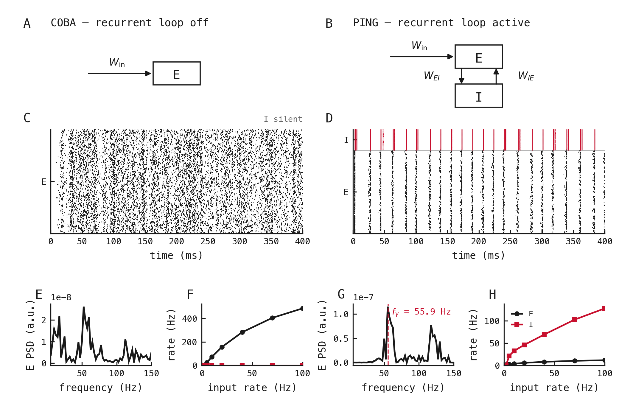
Figure 1: Loop-off and loop-on circuit architecture and activity. (A–B) Loop-off control and reciprocal E→I/I→E loop-on. (C–D) Illustrative 400-ms rasters: 1,024 E neurons (black), 256 I (red), and 1,024 Poisson channels at 5 Hz (loop-off) or 45 Hz (loop-on). (E, G) Mean-subtracted E-population Welch spectra; G’s dashed line marks the interpolated peak. (F, H) Mean per-neuron E/I rates over matched 2–100-Hz drive sweeps using the same 1,024-channel networks as the rasters and spectra. Each point is one single-seed trial, without uncertainty estimates; vertical scales differ. Source experiment: exp023 — Turning the PING Loop On.
P2
Loop-off excitatory spikes were dispersed, with silent inhibitory neurons (Fig. 1C); loop-on instead produced recurring E/I volleys and a 56.0-Hz spectral peak with higher-frequency harmonics, with loop-off lacked (Fig. 1D,E,G).
In matched 2–100-Hz drive sweeps on the same 1,024-input networks as the illustrative rasters, loop-off excitatory firing increased from 1.7 to 484.6 Hz while inhibition remained silent. Loop-on excitatory rates were constrained, staying between 1.7 and 11.6 Hz, while inhibitory firing reached 127.5 Hz (Fig. 1F,H).
P3
We next varied the strengths of both directions of the excitatory–inhibitory loop to examine how coupling affected firing rates and rhythmic activity. Across an 11×11 reciprocal-coupling grid, absent E→I or I→E coupling left excitatory firing near 169 Hz and autocorrelation lobe–trough contrast (Appendix B2) near zero (Fig. 2A–C). With both pathways present, stronger coupling reduced excitatory firing to single-digit rates, sustained inhibitory firing and increased contrast towards one across a broad region.
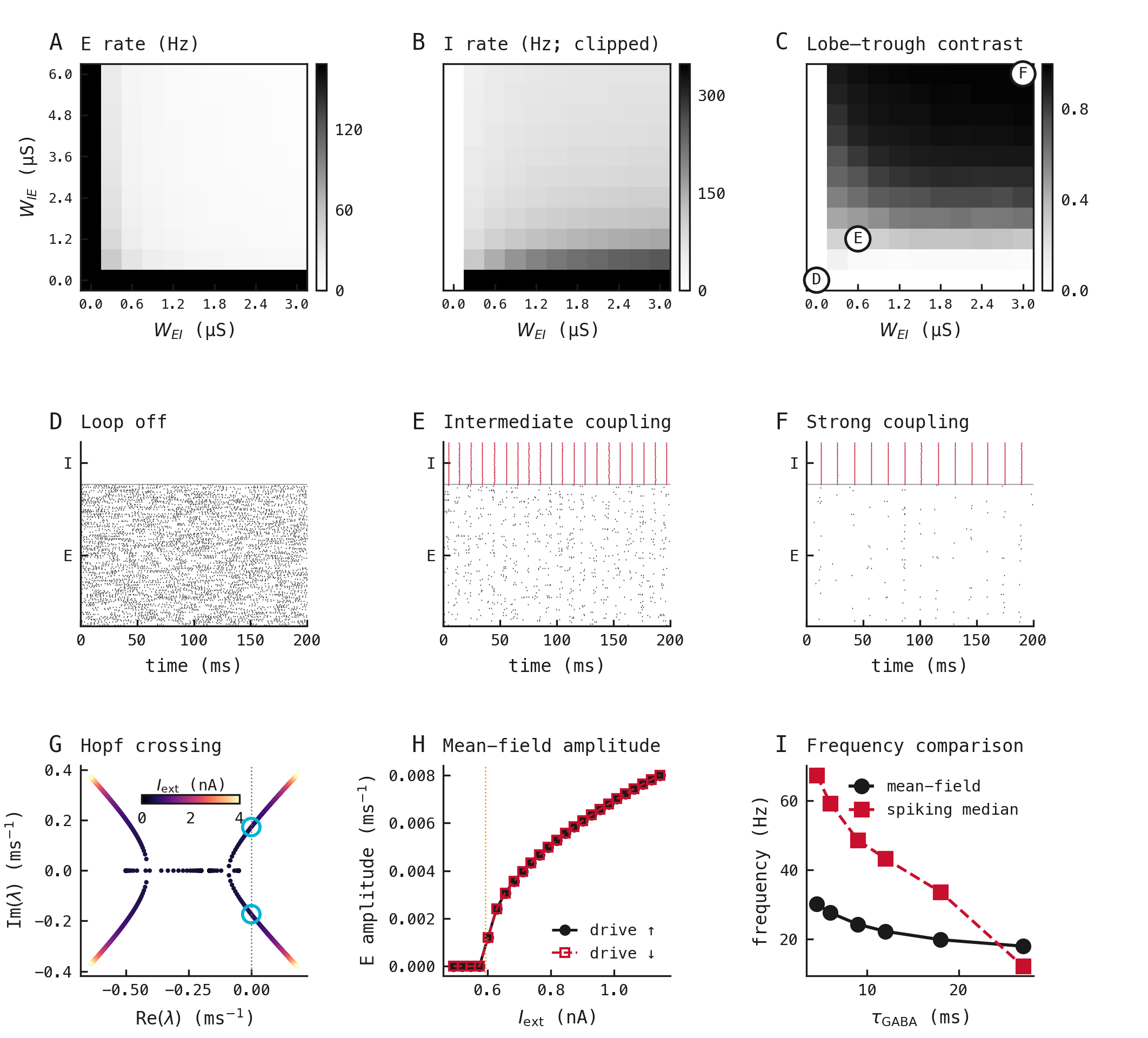
Figure 2: Reciprocal-coupling sweep and mean-field onset. (A–C) Mean E rate, I rate and autocorrelation lobe–trough contrast across an 11×11 grid of E→I () and I→E () initialization means on the fan-in-normalized summed-conductance scale. Each point represents one untrained network and seed; B’s grayscale is clipped at its 92nd percentile. (D–F) Illustrative 200-ms rasters at , and µS; black/red marks show 160 E/48 I neurons. A–F have no uncertainty estimates. (G–H) Separate four-variable mean-field model. G shows fixed-point eigenvalues across –4 nA (colour), with the leading pair at nA circled in cyan. H shows upward/downward peak-to-peak E-rate amplitudes; the dotted line marks onset. (I) Mean-field onset frequencies (black circles, solid) and median finite-drive spectral peaks from three separately trained classifiers (red squares, dashed), without uncertainty intervals. Methods define measurements and protocols. Source experiments: exp054 — Pinglab Rythmicity Metric, exp117 — Mean-Field Analysis of PING Bifurcations, and exp041 — Firing Rate Tracks Gamma Frequency.
P4
Selected rasters illustrate the same progression (Fig. 2D–F): autocorrelation contrast increased from 0.00030 without coupling to 0.268 at intermediate coupling and 0.989 at strong coupling, as excitatory firing became sparse and inhibitory volleys increasingly regular.
P5
We used a separate four-variable mean-field model to examine how oscillations emerged as external drive increased (Appendix C). Leading complex-conjugate eigenvalues crossed zero real part at nA, corresponding to 27.6 Hz (Fig. 2G). Above onset, excitatory-rate amplitude increased continuously, with nearly coincident upward/downward sweeps and no resolved hysteresis (Fig. 2H). A positive amplitude-squared slope and met the predefined numerical criteria for supercritical onset; criticality was not established analytically.
P6
We then compared how slowing inhibition affected oscillation frequency in the mean-field model and trained spiking classifiers. Increasing inhibitory decay from 4.5 to 27 ms reduced mean-field onset frequency from 30.2 to 17.9 Hz and median spiking-classifier spectral frequency from 67.3 to 12.2 Hz (Fig. 2I). The mean-field and spiking models showed the same qualitative behaviour—frequency decreased as inhibitory decay slowed. The comparison was intended to assess qualitative behaviour rather than establish quantitative agreement between mean-field onset eigenfrequencies and finite-drive spectral peaks.
The fixed reciprocal loop preserves accuracy at lower excitatory rates
P7
We next trained loop-on and loop-off networks to classify handwritten digits from MNIST using backpropagation through time with surrogate gradients, asking whether reciprocal inhibition could reduce excitatory firing while preserving classification accuracy. Both architectures reached approximately 90% validation accuracy, with dense loop-off firing and recurring loop-on volleys (Fig. 3A–C). Loop-on achieved 89.8% mean test accuracy at a mean excitatory firing rate of 16.6 Hz, versus 90.9% at 88.2 Hz for loop-off: a 5.3-fold firing-rate reduction and 1.1-percentage-point accuracy reduction (Fig. 3D). Tightening the activity-penalty ceiling progressively reduced excitatory firing and classification accuracy in both architectures, but their responses differed. Loop-off firing fell throughout the sweep, accompanied by a steeper loss of accuracy, whereas loop-on firing decreased less at the tightest ceilings while retaining higher accuracy. At the 1-Hz ceiling, loop-on averaged 4.7 Hz and 81.3% accuracy, compared with 2.1 Hz and 63.0% for loop-off. Thus, equal training ceilings did not generally produce matched firing rates. At the 10-Hz ceiling, however, both averaged approximately 9 Hz, with higher accuracy for loop-on (88.6% versus 83.5%).
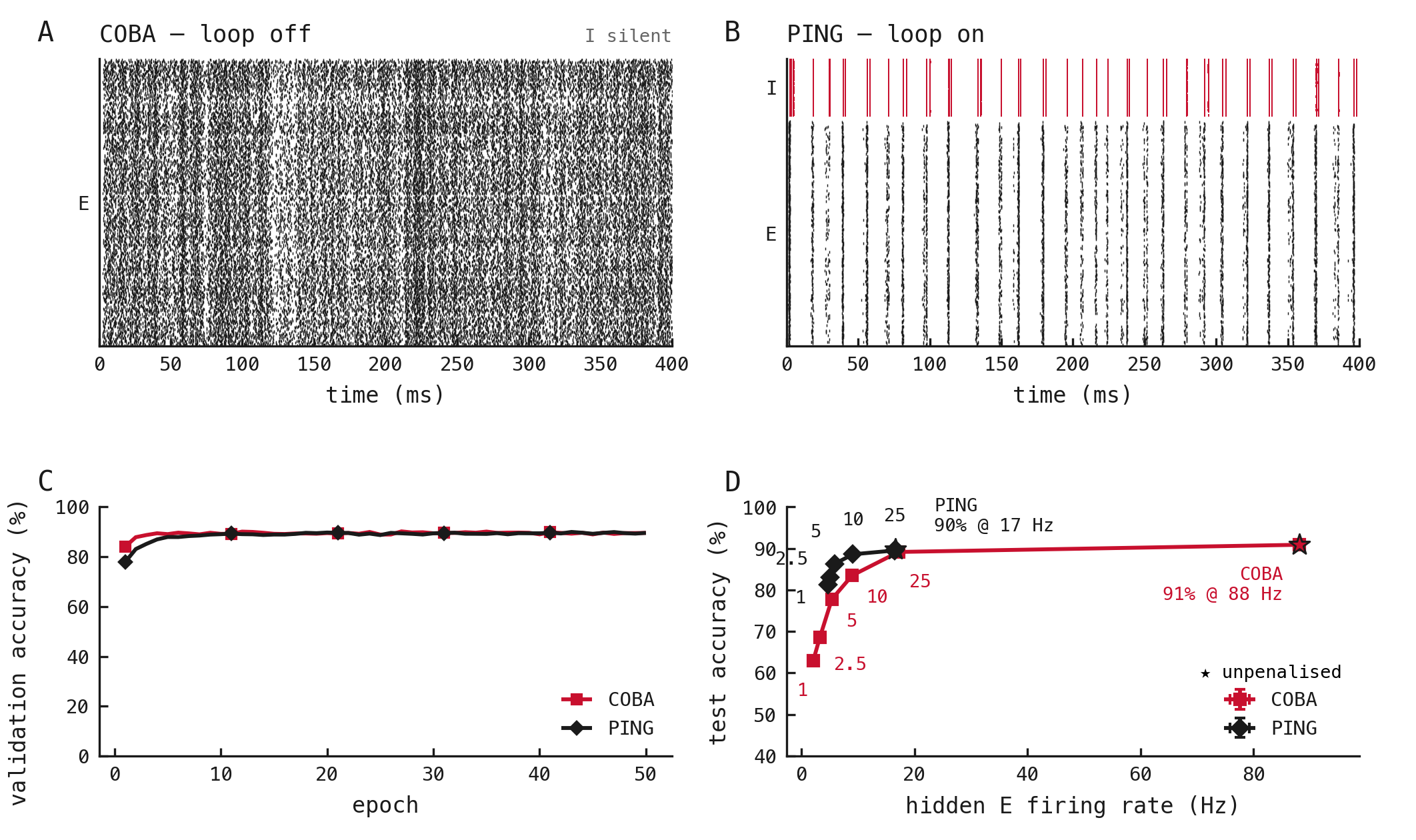
Figure 3: Accuracy and excitatory firing in loop-off and loop-on classifiers. (A–B) Illustrative 400-ms responses to digit-0 sample 0 from final unpenalised checkpoints, seed 42; E spikes are black, I red. (C–D) Loop-off: red squares; Loop-on: black diamonds. Means use three independent training replicates. C shows unpenalised validation accuracy without uncertainty intervals. D shows final-checkpoint test accuracy versus mean per-neuron E rate under the common endpoint protocol; bars show the standard error of the mean (SEM) on both axes. Ceilings were 1, 2.5, 5, 10 and 25 Hz; stars denote unpenalised conditions. The loop-on 25 Hz ceiling marker nearly coincides with its unpenalised star. Source experiment: exp025 — Accuracy and Firing Rate With and Without Inhibition.
P8
We next asked whether adding reciprocal inhibition after training could produce sparse rhythmic activity while preserving classification accuracy. Adding reciprocal inhibition to trained loop-off classifiers without retraining replaced dense excitatory activity with recurring E/I volleys (Fig. 4A,B). Across the coupling sweep, mean excitatory firing fell from 85.9 to 7.2 Hz (11.9-fold), inhibitory firing reached 40.0 Hz, and accuracy fell from 90.4% to 43.2% (Fig. 4C,D). The activity pattern therefore did not require learning with inhibition, but inserting the loop after training incurred a substantial classification cost.
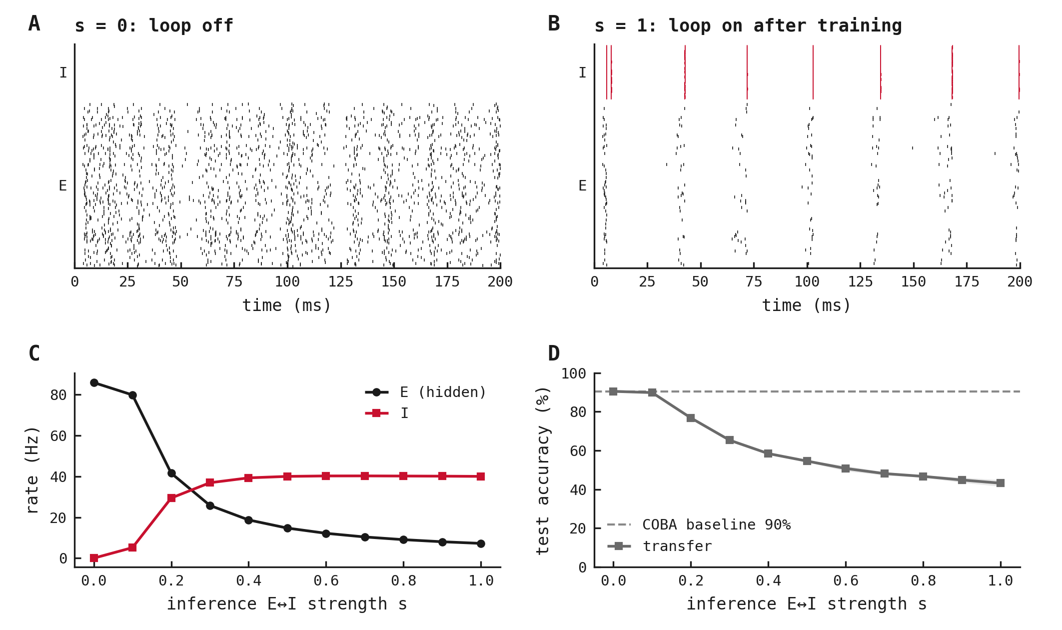
Figure 4: Post-training insertion of reciprocal inhibition. (A–B) Illustrative 200-ms responses to the same digit-7 image from one validation-selected loop-off classifier (seed 42), at and ; fixed pseudorandom subsets show 200 E neurons (black) and 64 I (red). Learned weights remained frozen; recurrent matrices were newly initialized at each strength without retraining (Methods). (C–D) Mean ± sample standard deviation (SD) across three independent classifiers, evaluated using the common endpoint protocol at –1 in 0.1 steps. C shows per-neuron E/I rates (black circles/red squares); D shows accuracy (grey squares), with the dashed line marking mean accuracy at . Source experiment: exp038 — Switching On the Inhibitory Loop.
P9
We next asked whether the rhythmic activity observed with fixed reciprocal coupling persisted when the recurrent excitatory–inhibitory weights were trained alongside the input and readout weights. Training recurrent weights reduced autocorrelation contrast relative to fixed loop-on recurrence. Final autocorrelation lobe–trough contrast was 0.999 with fixed recurrence, versus 0.094, 0.095 and 0.018 when recurrence was trained from standard, one-tenth-standard and zero initialization (Fig. 5C). These means describe three networks per condition responding to one fixed encoding of a reference digit, not test-set variability.
We also compared the recurrent connection weights before and after training. In all three networks in each condition, standard and one-tenth-standard training eliminated most E→I connections; most I→E connections remained positive and their mean strength across all entries increased (Fig. 5D–G). Mean E→I strength fell from standard but rose from one-tenth-standard initialization; zero-initialized recurrence remained zero. Weak contrast accompanied asymmetric reorganization in these three-replicate comparisons, without identifying a causal weight change.
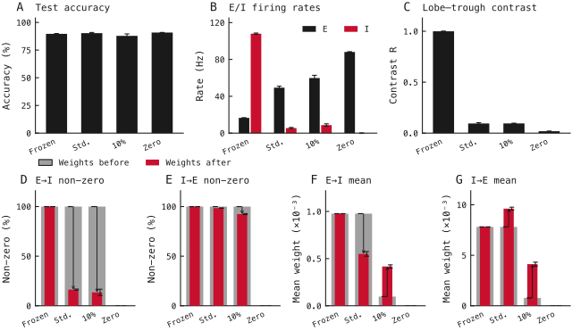
Figure 5: Epoch-50 activity, probe responses and recurrent weights. Input/readout weights were trained in four conditions: fixed recurrence (Frozen), or recurrence trained from standard (Std.), one-tenth-standard (10%) or zero (Zero) initialization. (A–B) Test accuracy and mean per-neuron E/I rates (black/red) under the common endpoint protocol. (C) Final, non-epoch-smoothed autocorrelation lobe–trough contrast from the same fixed digit-0, sample-0 encoding; this probe does not estimate trial-to-trial variability. A–C show means ± SEM across three independent training replicates. (D–E) Pooled positive-weight fractions for E→I/I→E. (F–G) Pooled arithmetic means including zeros, in µS. For each direction, condition and time point, the pool contains 786,432 entries from three equal-sized complete matrices, giving each network equal weight. Wide grey/narrow red bars denote initialization/epoch 50. Error bars show ±1 SEM across the three per-network statistics (sample SD divided by ), calculated separately before and after training; they do not describe uncertainty in the paired change. Individual weights are not independent training replicates. Arrows mark pooled relative changes ≥5%, not statistical significance. Source experiment: exp049 — Training Recurrent Weights Weakens PING Rhythmicity.
Excitatory firing is organised by population-cycle participation
P10
We next varied the inhibitory decay time in separately trained loop-on networks to examine how the timescale of inhibition shaped population rhythms, excitatory firing and classification accuracy. Across inhibitory decay times of 4.5–27 ms, mean spectral frequency fell from 67.5 to 11.7 Hz and excitatory firing from 18.3 to 2.8 Hz (Fig. 6A). The affine fit to six condition means had slope 0.285 Hz/Hz, intercept −0.70 Hz and . Mean test accuracy fell from 91.2% to 81.9% (Fig. 6B). Slower rhythms thus accompanied lower activity and a classification cost. The slowest condition lay below conventional gamma frequencies, so we describe the full sweep as population cycles rather than gamma cycles.[1]
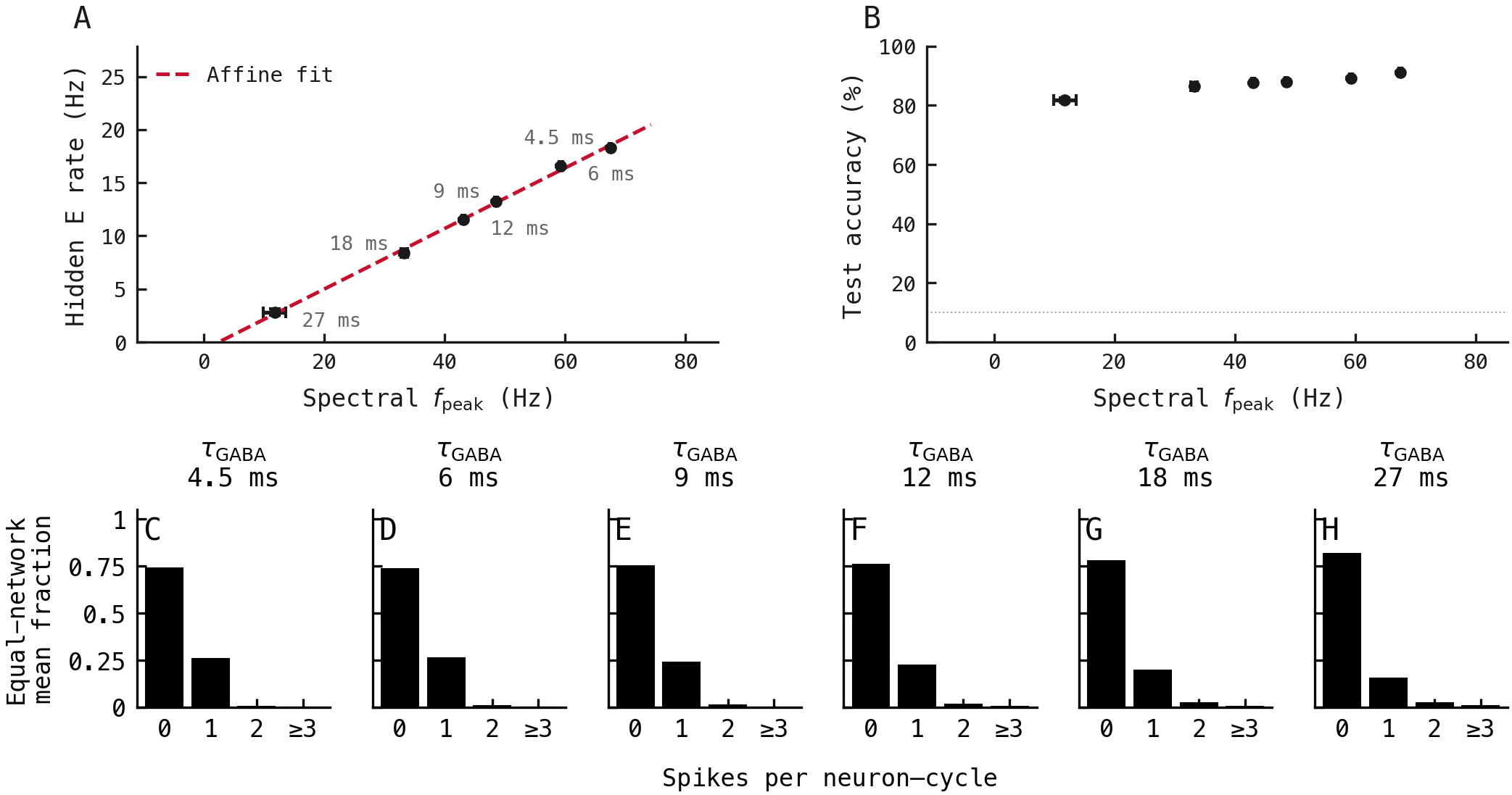
Figure 6: Excitatory firing and spike counts per cycle across inhibitory decay times. Eighteen epoch-50 classifiers comprise three independent replicates per decay time, evaluated with the common endpoint protocol. (A–B) Mean per-neuron E rate and test accuracy versus spectral-peak frequency , estimated from the largest interpolated 5–150-Hz peak of each network’s trial-averaged Welch spectrum. Points and both-axis bars show means ± SEM across replicates. Labels give decay times; A’s red dashed line is the equal-weight affine fit to six condition means. B’s dotted line marks 10% chance accuracy. (C–H) Equal-network mean fractions of E neuron–cycle pairs with 0, 1, 2 or ≥3 spikes at decay times 4.5, 6, 9, 12, 18 and 27 ms. Black bars show arithmetic means of the three networks’ separately normalized distributions, giving each network equal weight regardless of its detected cycle total; no uncertainty intervals are shown. Cycles span midpoints between detected inhibitory bursts, with edge intervals extending to presentation boundaries (Methods). Presentations without bursts are excluded. These distributions reuse the same classifiers’ recorded spikes without new inference or training. Source experiments: exp041 — Firing Rate Tracks Gamma Frequency and exp046 — One Spike per Gamma Cycle.
P11
To examine how individual neurons participated in these population rhythms, we counted each excitatory neuron’s spikes within cycles defined by successive inhibitory bursts. Across the 18 equally weighted networks, the mean fractions were 76.35% with no spikes, 22.09% with one spike and 1.56% with two or more: 98.44% contained at most one spike (Fig. 6C–H). These distributions support predominantly one-spike participation among active neurons alongside widespread within-cycle silence, without establishing a strict firing ceiling or constant participating fraction.
The operating regime has asymmetric perturbation sensitivity
P12
We next tested how loop-on and loop-off classifiers responded to disrupted spike transmission by deleting naturally generated spikes or inserting additional spike events during inference. Both networks maintained high accuracy when 80% of excitatory and inhibitory spike transmissions were randomly deleted: 88.9% for loop-off and 89.2% for loop-on. Deleting all transmissions reduced both to 10.6% (Fig. 7A). Adding extra spikes had a larger effect on loop-on networks. When spikes were added to both populations at each network’s baseline excitatory firing rate, accuracy fell to 76.4% for loop-off and 38.5% for loop-on. Doubling the rate of added spikes reduced accuracy further, to 53.1% and 11.4%, respectively (Fig. 7B). Loop-on therefore tolerated substantial deletion but was more sensitive to insertion at matched baseline-relative doses.
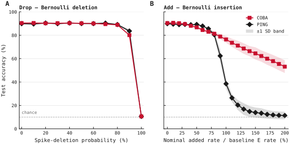
Figure 7: Spike perturbations in trained classifiers. (A–B) Inference-time perturbations of validation-selected unpenalised loop-off (red squares) and loop-on (black diamonds), without retraining, using the common endpoint protocol. Lines and shading show mean ± sample SD across three independent training replicates; dashed lines mark 10% chance accuracy. (A) Independent deletion of transmitted E/I spikes, preserving neuronal resets. (B) Independent insertion into both populations at 0–200% of each network’s unperturbed E firing rate; aggregation matches relative doses, not hertz. The same nominal per-neuron insertion rate applies to E and I. Collisions add no event; inserted events cause no reset or refractory period. Both interventions affect readout and recurrent transmission. Exact dose grids and operations are given in Methods. Source experiment: exp037 — Dropped Spikes vs Added Noise.
P13
We next examined whether classification performance depended on the simulation timestep by separately training and evaluating loop-on networks at five temporal resolutions. Classification accuracy remained near 90% across tested timesteps, although excitatory firing varied. This supports robustness after separate training at each timestep, without establishing fixed-weight convergence (Appendix A5).
P14
We next tested how inhibitory spike timing affected loop-on classifiers by artificially shifting and replaying recorded inhibitory spikes while preserving each neuron’s spike count within every presentation. Shifting each inhibitory spike separately reduced excitatory firing. Shifting all inhibitory spikes from the same fixed 22.8-ms time window together increased it (Fig. 8). At a proposed jitter standard deviation of 14 ms, independent shifts reduced mean excitatory firing from 16.6 to 0.0075 Hz and accuracy from 89.8% to 11.9%; group shifts increased firing to 68.3 Hz while accuracy declined to 82.5%. Replayed inhibitory firing remained 108.3 Hz. Thus, timing altered excitatory recruitment despite preserved inhibitory counts.
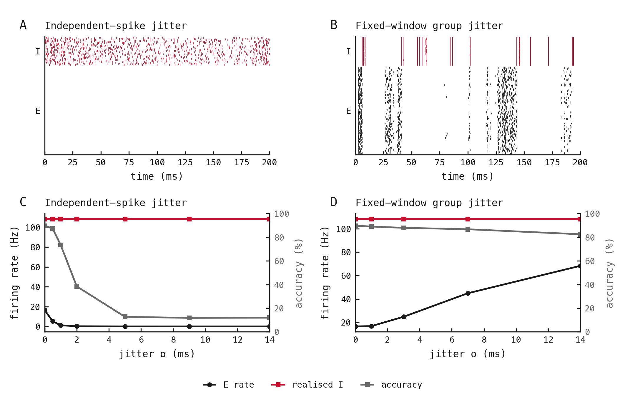
Figure 8: Count-preserving inhibitory replay perturbations. Recorded inhibitory spikes replace naturally generated outputs; excitatory activity and readout responses are recomputed with unchanged weights and inputs. (A–B) Illustrative digit-7 responses (test sample 0, seed 42) at proposed Gaussian-shift SD ms, showing the same 200 E neurons (black) and 64 replayed I neurons (red). (A, C) Independent-spike jitter. (B, D) Shared shifts within fixed 22.8-ms clock windows, defined independently of detected bursts. Grid rounding, reflection and collision handling preserve each neuron’s count (Appendix D). (C–D) Per-neuron E/I rates (black circles/red squares, left axes) and test accuracy (grey squares, right axes), averaged across three independently trained final-checkpoint classifiers using the common endpoint protocol; no uncertainty intervals. Displayed jitter values are 0, 0.5, 1, 2, 5, 9, 14 ms (C) and 0, 1, 3, 7, 14 ms (D); both share the zero-jitter replay control. Source experiment: exp042 — Inhibitory Replay Perturbations Change Excitatory Firing.
Loop-on networks classify continuously presented inputs
P15
We next tested whether loop-on classifiers could classify successive images while carrying their hidden state from one presentation to the next. A loop-on classifier trained across variable input rates correctly classified five successive digits presented at changing durations and input rates (Fig. 9A). Sparse excitatory firing (Fig. 9B) and inhibitory volleys (Fig. 9C) persisted throughout the stream. The readout accumulated spike-count evidence during each presentation (Fig. 9D). We selected an example in which all five digits were classified correctly; the first candidate met this criterion. The example therefore demonstrates feasibility, not reliability across arbitrary streams. Output state and counts reset at supplied boundaries, so this result does not establish autonomous boundary detection. We then evaluated streaming accuracy across different presentation durations and input strengths, using repeated trials to assess performance beyond the illustrative example. At 25-Hz maximum-pixel input, increasing duration from 25 to 200 ms raised mean accuracy from 75.2% to 90.3% (Fig. 9E). At 200 ms, increasing input from 0.5 to 5 Hz raised accuracy from 26.3% to 82.7% (Fig. 9F). Mean accuracy then increased across the tested rates from 5 to 25 Hz, reaching 90.3%. Brief presentations and weak drive constrained performance. The grid paired image identity and order across conditions; its uncertainty remains conditional on one sampled image bank.
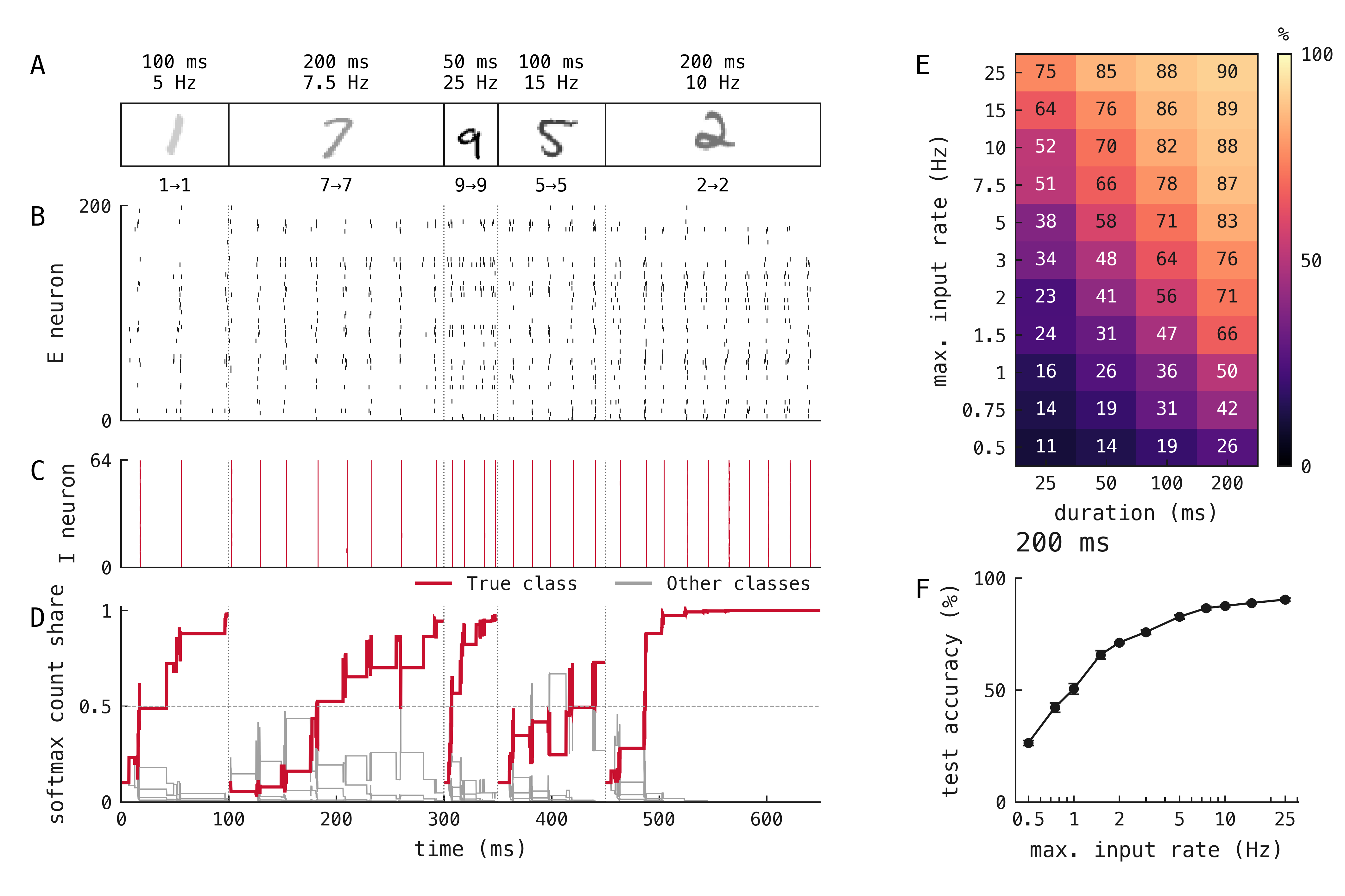
Figure 9: Spike-count classification in continuous MNIST streams. Three independently trained, validation-selected loop-on classifiers used variable-rate training (0.5–25 Hz). During inference, hidden E/I state continued between digits; output voltage/counts reset at supplied boundaries. (A–C) Reused illustrative seed-42 stream selected by a predefined five-correct criterion: digits 1, 7, 9, 5, 2 at duration–rate pairs (100 ms, 5 Hz), (200 ms, 7.5 Hz), (50 ms, 25 Hz), (100 ms, 15 Hz), (200 ms, 10 Hz). A shows images, labels and conditions; B/C show the first 200 E/64 I neurons (black/red). Dotted lines mark supplied boundaries. (D) Softmax-normalized cumulative output-spike counts: true class red, others grey. Shares are not calibrated probabilities; the dashed 0.5 line is not a decision threshold. Classification uses the largest final count (Methods). (E–F) Repeated quantitative evaluation on the same 40 ordered five-image streams for every network, duration and rate, with separate spike-encoding draws. Accuracy across 40 five-digit test streams per network/condition (200 decisions), with duration/rate fixed within each stream. E shows replicate-mean percentage accuracy at four durations and eleven rates, without uncertainty intervals. F reuses the 200-ms evaluations: mean ± SEM across three replicates on a logarithmic rate axis. The illustrative recording was selected separately from this grid. Source experiment: exp082 — Spike-Count Classification in a Continuous Stream.
Methods
Experimental design
P17
We combined untrained circuit simulations, trained MNIST classifiers, interventions on those classifiers and a separate mean-field model (Table 1). Inhibitory-timescale classifiers supplied frequency and cycle-participation measurements; unpenalised accuracy–rate classifiers supplied loop-insertion and spike-perturbation experiments. Unless specified otherwise, trained-network analyses used the common endpoint protocol below; Table 1 and Statistical reporting define checkpoints and replication.
| Figure | Design | Checkpoint |
|---|---|---|
| 1 | Untrained; 1,024 E, 256 I | — |
| 2A–F | Coupling grid; 1,024 E, 256 I | — |
| 2G–I¹ | Mean-field model | — |
| 3 | 2 architectures × 6 activity conditions | Final |
| 4 | Loop insertion; reused loop-off | Best validation |
| 5 | 4 recurrent-training conditions | Final |
| 6 2I² | 6 inhibitory decay times | Final |
| 7A–B | Spike perturbations; reused loop-off/loop-on | Best validation |
| App. A1 | 5 timesteps; 0.05–0.6 ms | Final |
| 8 | Inhibitory replay; reused loop-on | Final |
| 9 | Variable-rate, spike-count training | Best validation |
Table 1: Experimental design and checkpoint policy. E/I: excitatory/inhibitory neurons. Each training condition comprised three replicates. Final: epoch 50. Best validation: lowest mean validation cross-entropy across three encoding draws, with ties resolved by higher accuracy, then earlier epoch. ¹ Mean-field results. ² Spiking-model results.
Spiking networks
P18
Hidden excitatory and inhibitory neurons followed conductance-based leaky integrate-and-fire dynamics:
Here, is membrane voltage and is time. Membrane capacitance was 1 nF for excitatory neurons and 0.5 nF for inhibitory neurons; leak conductance was 0.05 and 0.1 µS, respectively. The leak reversal potential was −65 mV, while excitatory and inhibitory reversal potentials and were 0 and −80 mV. Synaptic conductances and varied with incoming spikes, as described below. At the spike threshold mV, neurons emitted a spike and returned to the reset potential mV. Voltage remained at reset for an absolute refractory period of 1.2 ms in excitatory neurons and 0.6 ms in inhibitory neurons.
P19
Synaptic conductances decayed exponentially and increased upon incoming spikes:
Here, is conductance at step , the conductance increment from source , and its delivered spike indicator. Decay times were ms and ordinarily ms. Exponential-Euler voltage integration used ms, except in the timestep study (Appendix A5). The inhibitory-timescale grid is specified below; exact updates and transmission ordering are in Appendix A1.
Spiking measurements used E/I refractory holds of 1.2/0.6 ms. The timestep comparison, separate mean-field calculation, quantitative continuous-stream evaluation and loop-off training and comparisons used the same refractory durations. The quantitative continuous-stream evaluation used a shared image bank.
P20
Classifier networks contained input→E, E→I, I→E and E→output projections, with E→E and I→I connections disabled; loop-off additionally disabled reciprocal E–I coupling. Input and recurrent weights used lower-clamped Gaussian draws with fan-in normalization (Appendix A4 Table A1). Here, is the presynaptic population size; input weights were initially zeroed with probability but remained trainable. Readout weights were dimensionless and initialized directly without fan-in normalization.
Classifier training
P21
MNIST images were flattened into 784-element vectors and their pixel intensities divided by 255. We sampled 7,000 images uniformly without replacement from the official training partition, then divided this subset into 6,300 optimization images and 700 validation images using a class-stratified split. Both sampling and splitting used seed 42, giving the same data partitions across training replicates. The official 10,000-image test partition remained separate from optimization and checkpoint selection. Endpoint evaluations in Figs. 3–8 and Appendix Fig. A1 used a common subset of 1,000 test images sampled uniformly without replacement using seed 42, without class stratification. This subset and its presentation order were fixed independently of training seed. Single-image probes and illustrative rasters used separately specified examples; continuous-stream evaluations sampled from the full official test partition, as described below.
P22
Each normalized pixel drove an independent Bernoulli spike channel:
Here, indicates an input spike from pixel at timestep , is its normalized intensity, and is its per-step spike probability. The maximum-pixel rate was ordinarily 25 Hz, and the integration timestep is expressed in seconds in this equation. Draws were independent across pixels, timesteps and presentations, with at most one spike per channel per step.
Independent image presentations lasted nominally 200 ms and began with freshly initialized hidden and output states. Training generated fresh encoding draws on each presentation. Endpoint encodings were matched across networks at common input settings, with independent perturbation randomness (Appendix B5). Variable input rates and state continuity between successive images in the streaming experiment are described below.
P23
The output layer contained ten leaky integrate-and-fire units, one per digit class. Each unit had a dimensionless state , where denotes the class, and an output decay time ms. Weighted excitatory spikes drove this state. At each timestep, a pre-reset state at or above the output threshold produced one spike, after which the threshold was subtracted from the state. Output units had no refractory period and began each independent presentation at zero.
For ordinary classification (Figs. 3–8 and Appendix Fig. A1), class logits and predictions were
Here, is pre-reset output state at step , the presentation’s step count, the class logit and the predicted digit. Exact output updates are in Appendix A streaming uses the spike-count readout below.
P24
We trained classifiers for 50 epochs using AdamW with learning rate , zero weight decay and minibatches of 256 images. The objective was mean cross-entropy, supplemented by the activity penalty described below where applicable. We used full, untruncated surrogate-gradient backpropagation through the complete temporal unrolling of every presentation in each minibatch.[2] Before each optimizer update, we clipped the global Euclidean gradient norm to a maximum of 1. Trainable connection weights were subsequently clamped below at zero.
Spikes remained binary during forward simulation. During backpropagation, the threshold derivative was replaced by the fast-sigmoid surrogate
where is the spike indicator, is the numerical distance from threshold—expressed in millivolts for hidden neurons and normalized units for output neurons—and the surrogate slope . Gradients through each hidden excitatory and inhibitory membrane increment were additionally divided by the dimensionless voltage-gradient damping divisor in both loop-on and loop-off. Damping altered backward derivatives, not the forward update rule; output updates were undamped. Exact gradient paths are specified in Appendix A3.
P25
For the accuracy–rate comparison (Fig. 3D), we added a one-sided quadratic penalty to the classification loss:
Here, is the objective, mean classification cross-entropy, the minibatch size and the presentation index. The excitatory rate is that presentation’s excitatory spike count divided by excitatory population size and duration in seconds. Division by makes the excess dimensionless. We used dimensionless penalty coefficient at ceilings of 1, 2.5, 5, 10 and 25 Hz; the unpenalised condition used . The penalty acts on each presentation before minibatch averaging and imposes no hard rate limit. Only input/readout weights were trained; recurrence stayed fixed, enabled in loop-on and disabled in loop-off.
P26
After each training epoch, we evaluated the 700 validation images using three independently seeded spike-encoding draws. The same encoding seeds were reused across epochs, keeping stochastic inputs fixed for checkpoint comparisons. For variable-rate classifiers, validation input-rate draws were also fixed across epochs. Cross-entropy and accuracy were averaged over validation images and encoding draws; the activity penalty was excluded from the validation loss.
Best-validation checkpoints minimized mean validation cross-entropy over epochs 1–50, with ties resolved by higher accuracy, then earlier epoch. Final checkpoints were from epoch 50. Table 1 specifies the checkpoint used for each analysis.
Untrained circuit experiments
P27
We compared untrained loop-off and loop-on circuits containing 1,024 excitatory and 256 inhibitory neurons (Fig. 1). Reciprocal E→I and I→E coupling was absent in loop-off and enabled in loop-on, using the initialization parameters specified in Table A1. Each simulation lasted 400 ms at a 0.1-ms timestep, beginning with membrane voltages of −65 mV and zero synaptic conductances; no burn-in interval was discarded. Illustrative rasters used 1,024 independent Poisson input channels at 5 Hz per channel for loop-off and 45 Hz for loop-on. The matched input–output sweeps reused the same 1,024-input networks and fixed weights within each loop condition, testing both architectures at 2, 5, 10, 20, 40, 70 and 100 Hz per channel. Each architecture–input condition comprised one trial with seed 42. Population firing rates were measured over the full trial, and spectra were calculated from the illustrative raster trials as described below.
P28
We mapped reciprocal coupling in untrained networks containing 1,024 excitatory and 256 inhibitory neurons (Fig. 2A–F). Each excitatory neuron received its own independent 100-Hz input channel through a fixed input weight of 0.5 µS. The E→I initialization parent mean ranged from 0 to 3 µS in 0.3-µS increments, and the I→E parent mean ranged from 0 to 6 µS in 0.6-µS increments, forming an grid. Recurrent weights used Gaussian draws with standard deviations equal to 10% of their respective means, followed by lower clamping at zero and division by presynaptic population size. Each grid condition comprised one network and one trial with seed 42. Simulations lasted 1 s at a 0.1-ms timestep, with an inhibitory decay time of 6 ms. We discarded the first 100 ms and measured population firing rates and excitatory-population autocorrelation contrast over the remaining 900 ms. Illustrative rasters show the first 200 ms after burn-in at three selected grid conditions.
Activity measurements
P29
Mean per-neuron firing rates in Fig. 1F,H, Fig. 2A,B, Fig. 3D, Fig. 4C, Fig. 5B, Fig. 6A, Fig. 8C,D and Appendix Fig. A1A were calculated as
where is the firing rate of population , is its total spike count, is its neuron count and is the observation duration in seconds, summed across presentations when pooling trials.
For spectral analysis, we formed each presentation’s excitatory-population trace by averaging binary spike indicators across neurons at each simulation step. We subtracted the trace mean and estimated its power spectral density using Welch’s method with a single Hann window spanning the full presentation. For the inhibitory-timescale classifiers in Fig. 2I and Fig. 6A, spectra were averaged across the 1,000 test presentations within each network before locating the largest peak between 5 and 150 Hz. The spectral-peak frequency was refined by parabolic interpolation (Appendix B1). The 200-ms presentations gave a frequency-bin spacing of 5 Hz.
The illustrative spectra in Fig. 1E,G instead used individual 400-ms trials, giving 2.5-Hz bin spacing. Their peak annotation additionally required inhibitory spiking; absence of a marker was not a statistical test for rhythmicity. Interpolation formulas and boundary cases are specified in Appendix B.
P30
We quantified excitatory-population temporal structure using autocorrelation lobe–trough contrast (Fig. 2C and Fig. 5C). Spikes were pooled across excitatory neurons into 1-ms count bins. We normalized and smoothed the uncentered autocorrelogram over lags up to 100 ms as specified in Appendix B2.
We identified the first local minimum at a lag of at least 2 ms and the maximum at positive lags preceding that minimum. Contrast was defined as
Here, and are the preceding maximum and first minimum of the smoothed autocorrelation. Coupling-grid contrast used the 900-ms post-burn-in interval; classifier contrast used the fixed reference-image presentation below. Appendix B specifies the feature-selection and boundary rules.
Mean-field calculation
P31
We examined oscillatory onset using a separate four-variable mean-field model (Fig. 2G–I). Its state comprised excitatory and inhibitory population rates and , excitatory conductance onto inhibitory neurons , and inhibitory conductance onto excitatory neurons :
Here, dots denote derivatives with respect to time in milliseconds; rates were expressed in and conductances in µS. The external current , measured in nA, drove only the excitatory population. The functions and mapped mean input current to steady-state firing rate using noisy leaky integrate-and-fire gains.
The rate-relaxation constants ms and ms matched the respective membrane time constants. Synaptic decay constants were ms and, unless varied, ms. Fixed driving-force magnitudes were mV and mV; summed conductance increments were µS and µS. The gains used the leak, reset and threshold parameters specified above, refractory periods ms and ms, and an effective voltage-noise scale mV.
This phenomenological closure fixed synaptic driving forces at rest, omitted conductance-dependent shunting and assumed a noise scale that was neither measured nor fitted to spiking activity. The population equations were deterministic; noise entered through the gain functions. The gain integral and closure assumptions are specified in Appendix C.
P32
We continued fixed points across external currents –4 nA and located onset at , where the leading complex-conjugate eigenvalue pair first crossed from negative to nonnegative real part (Fig. 2G). Eigenvalues came from the continuous-time Jacobian of the four-variable model; continuation and refinement details are given in Appendix C2. The onset frequency was
Here, is either eigenvalue of the refined crossing pair and its imaginary part in radians per millisecond; is in hertz. The factor 1000 converts cycles per millisecond to hertz. Numerical settings are specified in Appendix C.
P33
We assessed criticality with 2-s upward/downward drive integrations, measuring peak-to-peak E-rate amplitude in over the final 500 ms at 1,001 fixed sample times (Fig. 2H). Numerical supercriticality required no resolved hysteresis and a positive amplitude-squared slope, using Appendix C’s predefined thresholds. No first Lyapunov coefficient was calculated, so narrower bistability or an unstable periodic orbit was not excluded. We repeated onset refinement at the six inhibitory decay times used for spiking classifiers, holding other mean-field parameters fixed. Fig. 2I compares the mean-field Hopf eigenfrequency with the median finite-drive spectral-peak frequency across three spiking classifiers per decay time.
Classifier comparisons and recurrent coupling
P34
We compared loop-off and loop-on under the six activity conditions defined above, giving 36 networks (Fig. 3). Final-checkpoint test accuracy and excitatory firing rates used the common endpoint protocol. Unpenalised validation learning curves averaged replicate accuracies at each epoch; illustrative-example selection is specified in Appendix B4.
The accuracy–rate, loop-insertion and spike-perturbation evaluations used the 18 loop-off classifiers trained with , together with the corresponding loop-on classifiers where applicable (Fig. 3, Fig. 4 and Fig. 7). The remaining classifier measurements used the networks and evaluation protocols specified in Table 1.
P35
We inserted reciprocal inhibition into the unpenalised loop-off classifiers from the accuracy–rate comparison, holding learned input and readout weights fixed without retraining (Fig. 4).
The dimensionless loop strength ranged from 0 to 1 in increments of 0.1. At each strength, we newly initialized the E→I and I→E matrices from Gaussian distributions with parent means µS and µS, respectively, and standard deviations equal to 10% of each mean. We clamped negative draws to zero and divided weights by the presynaptic population size: 1,024 for E→I and 256 for I→E. Thus, disabled the loop and used the standard recurrent initialization.
At each strength, we measured endpoint accuracy and E/I firing rates.
P36
We compared fixed recurrence at standard strength with trainable recurrence initialized at , or (Fig. 5), giving 12 networks. All conditions trained input and readout weights without an activity penalty. Endpoint accuracy and E/I firing rates used the common protocol. Contrast used the final training diagnostic from one 200-ms encoding of the first official-test digit-0 image, generated with seed 0 and fixed across networks, without smoothing across epochs.
For recurrent-weight comparisons, initial matrices were reconstructed using the original initialization seeds and parameters. At initialization and epoch 50, we pooled the three complete matrices separately for each connection direction and condition, giving 786,432 entries per pooled distribution. We calculated the fraction of strictly positive weights and the arithmetic mean weight across all entries, including zeros. Because the three matrices had equal size, each network contributed equally to these pooled summaries. We also calculated the same two statistics separately for each network and calculated their SEM across the three networks, separately at initialization and epoch 50. These were descriptive summaries, without significance tests of training-induced weight changes. Jointly trained weights within a matrix were not independent training replicates.
Inhibitory timescale and cycle participation
P37
We separately trained 18 loop-on classifiers at inhibitory decay times and ms (Fig. 6A–B). Input and readout weights were trained without an activity penalty; recurrence remained fixed at standard strength. Evaluation retained each assigned decay time and measured endpoint accuracy, excitatory firing rate and spectral-peak frequency using the common protocols.
We fitted the affine relationship
by ordinary least squares, giving equal weight to each of the six condition means. Here, and are the across-replicate mean excitatory firing rate and spectral-peak frequency, both in hertz; is the fitted intercept in hertz and is the dimensionless fitted slope. Fit quality was quantified by the coefficient of determination , using the centered total sum of squares. The mean-field comparison in Fig. 2I used medians of the same three per-network frequencies at each decay time.
P38
We reused the same classifiers’ recorded spikes to measure excitatory counts per cycle (Fig. 6C–H), without new inference or training. Inhibitory bursts were detected from smoothed population counts with peak separation scaled to each network’s spectral period (Appendix B3).
Cycle boundaries were midpoints between inhibitory-burst peaks, with edge intervals extending to presentation boundaries. Presentations without bursts were excluded. Each excitatory neuron–cycle pair was classified as containing 0, 1, 2 or ≥3 spikes. We normalized each network’s four counts separately across its presentations and averaged its fractions equally with the other two networks in its condition, or across all 18 networks for the overall summary. This gave each network equal weight irrespective of its detected cycle total and balanced the six decay conditions in the overall summary. Appendix B specifies discretization and single-burst conventions.
Spike perturbations and numerical resolution
P39
We separately applied deletion and insertion to unpenalised loop-off and loop-on classifiers without retraining (Fig. 7A–B), using the common endpoint protocol and matched input encodings across perturbation conditions.
Deletion independently suppressed each naturally generated excitatory or inhibitory spike with probability , preserving the neuronal reset and refractory period associated with that spike.
For insertion, we first measured each network’s unperturbed mean per-neuron excitatory firing rate, , across the complete test subset. The nominal per-neuron insertion rate was , where the dimensionless dose . Independent Bernoulli events were sampled for every excitatory and inhibitory neuron at each timestep, with probability equal to the insertion rate in hertz multiplied by the timestep in seconds. The same nominal insertion rate applied to both populations. Transmission was capped at one spike per neuron per timestep, so insertion coinciding with an existing spike added no event. Inserted events triggered neither resets nor refractory periods.
Modified events supplied the readout and subsequent recurrent transmission. Insertion conditions were aggregated at matched baseline-relative doses.
P40
We evaluated separately trained loop-on classifiers at matched training and evaluation timesteps while holding refractory durations fixed. The full protocol and results are given in Appendix A5.
P41
We applied two count-preserving inhibitory replay perturbations to unpenalised loop-on classifiers (Fig. 8). Unperturbed inhibitory spikes recorded under the common endpoint protocol were shifted and replayed, replacing naturally generated inhibitory outputs while excitatory activity and readout responses were recomputed with unchanged weights and identical inputs.
For the conditions reported in Fig. 8, independent-spike jitter assigned each inhibitory event a zero-mean Gaussian offset with standard deviation or ms. Group jitter assigned one shared Gaussian offset to all inhibitory events originating within each fixed 22.8-ms window of a presentation, using or ms. These windows comprised 228 simulation steps and were defined independently of detected bursts.
Each inhibitory neuron’s spike count was preserved within every presentation. The parameter describes proposed offsets before boundary and collision adjustments; both arms shared the zero-jitter replay control. Exact transformations are specified in Appendix D.
We measured endpoint accuracy and excitatory and replayed inhibitory rates. Delivered inhibition could not respond to ongoing excitatory activity.
Continuous streams
P42
Continuous-stream classifiers used the common isolated-image training protocol without an activity penalty, training input and readout weights while keeping recurrence fixed at standard strength (Fig. 9).
For each presentation, the maximum-pixel input rate, , was sampled uniformly from 0.5, 0.75, 1, 1.5, 2, 3, 5, 7.5, 10, 15 and 25 Hz and held constant throughout that presentation. Rates were sampled independently for individual images within each minibatch and resampled on subsequent presentations.
Continuous-stream classifiers used the output units defined above, with class logits given by accumulated spike counts:
Here, indicates an output spike; class index , logit and presentation length are defined above. Counts entered cross-entropy directly without decay or duration normalization, using the same surrogate derivative. Classification selected the largest final count, breaking ties by lowest class index.
Readout weights were drawn from a Gaussian distribution with dimensionless mean and standard deviation , then clamped below at zero, without fan-in normalization. Evaluations used each network’s best-validation checkpoint with weights held fixed. The same three validation-selected classifiers were evaluated across all duration–rate conditions. During continuous streams, output state and accumulated counts were reset to zero at each supplied image boundary, while hidden neuronal and synaptic states continued between images.
P43
For quantitative streaming evaluation (Fig. 9E–F), we crossed presentation durations of 25, 50, 100 and 200 ms with the eleven maximum-pixel input rates used during training. Each of the three frozen classifiers processed 40 five-image streams per duration–rate combination, in batches of five streams. This gave 200 classification decisions per network and condition, and 26,400 decisions overall. Duration and input rate remained constant within each stream, and images followed without gaps. Each stream began with freshly initialized hidden and output states; subsequent image boundaries used the state-handling procedure described above.
For each stream, five images were sampled uniformly without replacement from the full 10,000-image official MNIST test partition, without class stratification. Digit labels could repeat within a stream, and images could recur across streams. We prespecified one bank of 40 ordered streams and reused the same image indices for every network, duration and rate. Thus, conditions shared both the target images and the preceding-image order. Spike encoding used separate generators with distinct seeds for all 5,280 network–condition–stream combinations (Appendix B5). The 26,400 decisions are repeated evaluations of this image bank, not that many independently sampled images.
Accuracy included all 200 decisions per network and condition, including presentations with no output spikes. Fig. 9F reuses the 200-ms evaluations from Fig. 9E aggregation and uncertainty follow the reporting protocol below. Presentation and count-accumulation windows had equal duration, so their effects were not separated. We did not compare continuing hidden state with a hidden-state-reset control or test autonomous image segmentation.
P44
We reused the illustrative recording selected independently of quantitative evaluation using a predefined five-correct criterion, met by the first candidate (Appendix B4). It was not a stream from the shared quantitative image bank.
To visualize the evolving readout within each presentation, we transformed cumulative output-spike counts into softmax shares:
Here, counts class- output spikes through step since the supplied boundary; is its dimensionless share, with indexing classes. These uncalibrated shares visualize evidence; the 0.5 line is not a decision threshold.
Statistical reporting and reproducibility
P45
For trained-network comparisons, the unit of replication was one separately initialized and trained network, with three replicates per condition (seeds 42–44). These seeds controlled network initialization and, for variable-rate training, the sampling of input rates. The training-data split and endpoint test-image subset were fixed separately. Repeated interventions on a network were repeated measurements; individual weights, neurons, presentations and neuron–cycle pairs were not additional network replicates. Untrained circuit probes used a single seed, and mean-field calculations were deterministic.
Each network’s outcome was calculated before aggregation across networks. Displayed error bars or bands represent SEM in Figs. 3, 5A–G, 6A–B and 9F and Appendix Fig. A1, and sample SD in Figs. 4 and 7A–B. Sample SD used the denominator , and SEM was calculated as , where is the number of training replicates.
For continuous-stream evaluation, all networks shared one image bank but used different encoding draws. Its SEM therefore summarizes variation across these trained networks and their encodings, conditional on the sampled images. One bank and one encoding draw per network, condition and stream do not separately estimate image-sampling, encoding and training variability. Image pairing does not make the 200 sequential decisions per condition independent network replicates.
Figures 8 and 9E show means without uncertainty intervals. Pooled weight summaries gave equal weight to each network because the matrices were equal-sized; their SEM used the three network-level summaries. Equal-network neuron–cycle distributions averaged separately normalized network fractions. These were descriptive means without uncertainty intervals. These summaries and fitted relationships do not treat neuron–cycle pairs as independent replicates.
Cycle-participation analysis excluded twelve of 18,000 presentations without a detected inhibitory burst, all from the seed-43 network at 27-ms inhibitory decay. These presentations contained excitatory activity, but it was too dispersed to recruit the inhibitory population. The affected images provided unusually weak input, while this network also had comparatively weak input connections and low firing rates. Because the same images recruited inhibition in the other network replicates, the failures appear to reflect a combination of weak stimuli, network-specific properties and stochastic encoding rather than a single cause.
All 84 included networks completed 50 training epochs.
P46
Spiking simulation, training and evaluation used custom Python/PyTorch code; all 84 classifiers were trained with PyTorch 2.11.0+cu128 on CUDA devices. Mean-field calculations used Python 3.10.19, NumPy 2.2.6 and SciPy 1.15.3. Experiment records retain stage-specific parameters, seeds, software/source revisions and original provenance for reused classifiers.
Supplementary details
Appendix A — Discrete dynamics and gradient calculations
A1 — Discrete neuronal and synaptic updates. These updates governed the spiking circuits in this study; their standard parameters are listed in Table A1. Let denote the number of completed updates. We updated conductances using Equation 2, first applying exponential decay and then adding the full weighted spike increments. Both recurrent pathways used spikes emitted during the preceding update; current external input entered the excitatory conductance before voltage integration. Consequently, newly emitted E or I spikes first affected the partner population in the following update.
For each neuron, the updated conductances defined the total conductance and effective equilibrium voltage:
Holding these conductances constant over the step, we calculated the trial voltage
Here, is in µS, and and are voltages in mV. The numerical lower bound mV guarded against extreme negative values: any calculated voltage below this bound was replaced by −200 mV before spike evaluation. Membrane capacitance , timestep , leak conductance , synaptic conductances , and reversal potentials retain their Methods definitions.
After calculating the trial voltage, we decremented the integer refractory counter by one, with a lower bound of zero. A neuron emitted a spike only when the decremented counter was zero and . Spiking or still-refractory neurons were assigned the reset voltage mV; otherwise, the trial voltage was retained. Each spike reloaded the counter with , where is the population-specific refractory duration and was an integer at every tested timestep. Spike eligibility therefore resumed on the -th subsequent update. Conductances continued evolving during refractory holds.
A2 — Output-state recurrence. We updated each output unit after the hidden population, using excitatory spikes delivered during the same timestep. With the indexing of Appendix A1, the pre-reset state, output spike and retained state were
Here, is the dimensionless weight from hidden excitatory neuron to output class , and denotes its delivered spike. The decay factor was , where is the output decay time. The dimensionless quantity expresses the timestep numerically in milliseconds and specifies the input-scaling convention. The indicator equals one when its condition holds and zero otherwise; is the output threshold. Only one threshold was subtracted per update, so the retained state could remain above threshold after a spike.
The readout modes differed in the quantity accumulated before this subtractive reset. Mean-state readout accumulated the pre-reset state for Figs. 3–8 and Appendix Fig. A1, whereas spike-count readout accumulated the emitted spike for Fig. 9:
Here, is the cumulative pre-reset state and the cumulative output-spike count. Neither accumulator decayed. The final logits were or , respectively, where is the presentation’s step count. Output state and accumulators began at zero; supplied image-boundary resets cleared them before that step’s output drive was applied.
A3 — Surrogate and damped derivatives. These derivatives governed the classifier training underlying Figs. 3–9 and Appendix Fig. A1. Spikes used the binary forward threshold and surrogate backward derivative in Equation 5. To implement voltage-gradient damping, we used a stop-gradient operator , which returned but contributed zero derivative during backpropagation. We defined
where is the damping divisor. We used in both loop-on and loop-off. This operation preserved the forward value while multiplying its backward derivative by .
For both hidden populations, we applied this operation to the exponential-Euler membrane increment from Appendix A1, before voltage clipping and reset:
Here, denotes voltage before clipping. Damping scaled every derivative through , including its dependence on conductances and previous voltage, while the additive path retained unit derivative. At fixed updated conductances, the resulting backward rule was
The subscript BP identifies the derivative used by backpropagation; timestep, total conductance and capacitance retain their Appendix A1 definitions. Conductance recurrences and the surrogate spike function received no separate damping factor.
Hidden reset and refractory decisions used Boolean masks and integer counters that were not differentiated. The retained-voltage branch carried zero derivative when a neuron spiked or remained refractory, while the spike-output branch retained surrogate gradients whenever the refractory mask permitted spiking. Voltage clipping also blocked gradients below the numerical floor.
Output updates received no voltage-gradient damping. Their subtractive reset retained the derivative through the output spike, giving
where denotes the surrogate derivative in Equation 5 and the output-state symbols retain their Appendix A2 definitions. The current-step accumulator increment contributed a direct derivative for mean-state readout and a surrogate derivative for spike-count readout.
A4 — Initialization transformation. For each input or recurrent projection, we generated independent Gaussian draws and Bernoulli retention indicators, then formed the initial weights:
Here, rows index presynaptic neurons, columns index postsynaptic neurons, and is the presynaptic population size. The parent mean and standard deviation follow the projection-specific parameters in Table A1; and are conductance increments in µS. Input connections used , giving a retention-compensation factor of 20; recurrent connections used . Negative Gaussian draws produced additional zeros through lower clamping.
Writing for the mean after lower clamping, this transformation gave
Thus, compensation for zeroing preserved the expected summed incoming weight after lower clamping. Parent parameters described the Gaussian before these transformations; realised matrix means and incoming sums additionally depended on finite sampling and Bernoulli zeroing. The retention mask was used only during initialization, so initially zero trainable weights could become positive during optimization.
Readout weights followed a separate initialization:
Here, indexes output classes. These weights were dimensionless and used no additional Bernoulli zeroing or fan-in normalization. Their parent mean and standard deviation follow Table A1 for ordinary classification and the continuous-stream Methods for streaming classifiers.
| Parameter | Standard value |
|---|---|
| Population sizes | 1,024; 256 |
| Membrane capacitance , E/I | 1/0.5 nF |
| Leak conductance , E/I | 0.05/0.1 µS |
| Leak/reset potentials | −65 mV |
| Spike threshold | −50 mV |
| Reversal potentials | 0; −80 mV |
| Refractory period , E/I | 1.2/0.6 ms |
| Synaptic decay | 2; 6 ms |
| Integration timestep | 0.1 ms |
| Input parent mean/SD | 0.9/0.09 µS |
| Recurrent parent mean/SD, E→I | 1/0.1 µS |
| Recurrent parent mean/SD, I→E | 2/0.2 µS |
| Input-zeroing probability | 0.95 |
| Readout initialization mean/SD (dimensionless) | 1.12/0.835 |
| Output decay time; threshold | 2 ms; 1 |
| Presentation duration; maximum-pixel rate | 200 ms; 25 Hz |
| Optimizer; learning rate | AdamW; 0.0004 |
| Epochs; minibatch size | 50; 256 |
| Weight decay; gradient-norm limit | 0; 1 |
| Surrogate slope; voltage-gradient damping | 1; 1,000 (loop-on and loop-off) |
Table A1: Standard spiking-classifier parameters and exceptions. Values describe standard classifiers, not the separate mean-field model. Fig. 1 used input parent mean/SD 1.5/0.3 µS and loop-on recurrent means 1.5/3 µS. Coupling strengths, inhibitory decay times and timesteps varied in their respective sweeps. Fig. 9 used readout mean/SD 0.05/0.04 and variable input rates; stream durations varied during evaluation. Readout initialization values are rounded.
A5 — Timestep dependence after separate training.
We assessed timestep dependence using 15 loop-on classifiers: three training replicates (seeds 42–44) at each integration timestep of 0.05, 0.1, 0.2, 0.3 and 0.6 ms. All networks underwent 50 training epochs without an activity penalty, with recurrent weights fixed at standard strength. Three existing 0.1-ms classifiers were reused; twelve networks were trained at the remaining timesteps. Excitatory and inhibitory refractory periods remained 1.2 and 0.6 ms, respectively, corresponding to integer step counts throughout.
Each epoch-50 checkpoint was evaluated at its training timestep on the common 1,000-image test subset. Nominally 200-ms presentations were truncated to complete simulation steps, giving realised durations of 199.8 ms at 0.3 and 0.6 ms and 200 ms otherwise. Mean per-neuron excitatory firing rates included all excitatory neurons and test presentations, using the realised duration. Accuracy and firing rate were summarised as means and SEM across the three training replicates at each timestep.
Mean test accuracy ranged from 88.37% to 89.63% across the twelvefold timestep range (Appendix Fig. A1). Mean excitatory firing was 14.27 Hz at the finest timestep and 17.02 Hz at the coarsest. Classification performance therefore persisted across the tested resolutions, while excitatory activity remained timestep-dependent. Because each network was trained and evaluated at the same timestep, this comparison combines timestep effects during training and evaluation; it does not establish numerical convergence with fixed weights.
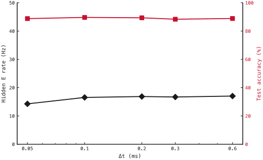
Figure A1: Timestep dependence after separate training. Mean per-neuron excitatory firing rate (black diamonds, left axis) and test accuracy (red squares, right axis) versus integration timestep on a logarithmic horizontal axis. Points show means across three independently trained loop-on classifiers per timestep (seeds 42–44); error bars indicate ±1 SEM. Epoch-50 checkpoints were evaluated at their training timestep on the same 1,000 MNIST test images. Firing rates use realised presentation durations: 199.8 ms at 0.3 and 0.6 ms, and 200 ms otherwise. Source experiment: exp044 — Firing Rate Across the Timestep Sweep.
Appendix B — Measurement algorithms and boundary cases
B1 — Spectral interpolation. This refinement supplied the spectral frequencies in Fig. 1E,G, Fig. 2I and Fig. 6A. We refined the spectral maximum using a parabola through three neighbouring bins of linear power spectral density. Let index the largest-power bin within the search interval, choosing the lowest-frequency bin when maxima were tied. The interpolated spectral-peak frequency was
Here, is the power spectral density at frequency bin , is the selected bin’s frequency, is the frequency-bin spacing in hertz, and is a dimensionless offset. Clipping limits the displacement to half a bin.
Neighbouring bins could lie outside the search interval, and the interpolated frequency was not subsequently restricted to that interval.
B2 — Autocorrelation implementation. This algorithm supplied the lobe–trough contrasts in Fig. 2C and Fig. 5C. We pooled excitatory spikes across neurons into complete 1-ms population-count bins, discarding any incomplete final bin. The dimensionless, uncentered autocorrelogram was
Here, is the excitatory population spike count in bin , is the number of complete bins, is their mean count, and is the lag in milliseconds.
We computed the numerator by zero-padding the count sequence to the smallest power-of-two length of at least , then inverse-transforming the squared magnitude of its fast Fourier transform. The padding prevented circular wraparound. Division by corrected for the decreasing number of overlapping bin pairs at longer lags, while division by removed the overall firing-rate scale. Approximately independent stationary counts therefore had a baseline near one.
We excluded zero lag because it was dominated by spikes matching themselves. Before smoothing, we replaced this entry with its 1-ms neighbour and convolved the autocorrelogram with weights , using zero padding beyond both ends. This reduced small finite-sample fluctuations during feature selection.
Denoting the smoothed values by , we selected the first lag satisfying and . The lobe was the maximum at positive lags preceding this trough, with ties resolved by the earliest lag. These values entered the contrast equation in Methods.
B3 — Burst detection and cycle-boundary discretization. This procedure supplied the equal-network neuron–cycle distributions in Fig. 6C–H. For each presentation, we summed inhibitory spikes across neurons at each 0.1-ms simulation step and convolved the resulting trace with a unit-sum Gaussian kernel of standard deviation 1 ms. The kernel extended ±4 ms (81 samples), with zero padding beyond the presentation boundaries. Candidate bursts were interior local maxima reaching at least 5% of the maximum smoothed value within that presentation. Flat maxima were represented by their middle sample, rounded down for even-length plateaus. Minimum peak separation was half the period corresponding to the network’s spectral-peak frequency , converted to simulation steps and rounded down, with a minimum of one step. Smaller competing peaks were removed first. The same network-level frequency set this separation for every presentation.
For consecutive detected peak indices and , we placed the intervening boundary at
where is an integer simulation-step index and the floor operation rounds downward. The outer boundaries were zero and , the presentation’s number of simulation steps. Excitatory spikes were counted separately for each neuron in the resulting half-open intervals: the starting boundary was included and the ending boundary excluded. A spike at an internal boundary therefore belonged to the following interval. The first and last intervals extended to the presentation boundaries and could contain partial cycles. When only one burst was detected, its counting interval covered the entire presentation; presentations without detected bursts contributed no neuron–cycle pairs.
B4 — Illustrative-example selection.
For Fig. 3, illustrative rasters used the seed-42, epoch-50 checkpoint from each architecture and the first digit-0 image in the official test set, presented for 400 ms.
For Fig. 4, illustrative rasters used the seed-42 classifier and the first image in the official test set, a digit 7, at and . Both presentations lasted 200 ms. Fixed subsets of 200 E and 64 I neurons were selected uniformly without replacement using seed 0 for display.
For Fig. 8, illustrative rasters used the seed-42 classifier and official test image 0, a digit 7, at ms.
For the illustrative stream (Fig. 9A–D), we used the seed-42 classifier with five predefined presentation-duration–maximum-pixel-rate pairs: (100 ms, 5 Hz), (200 ms, 7.5 Hz), (50 ms, 25 Hz), (100 ms, 15 Hz) and (200 ms, 10 Hz). Each candidate contained five distinct digit classes drawn in random order, with one image sampled uniformly from each class in the official MNIST test partition.
Candidates were evaluated in a predetermined order, and the first yielding five correct classifications was retained for the illustration. The first candidate met this criterion, producing the sequence 1, 7, 9, 5 and 2. Its image-selection and spike-encoding seeds were 820000 and 830000, respectively. This illustrative selection was separate from the quantitative streaming evaluation. Rasters displayed the first 200 excitatory and 64 inhibitory neurons.
B5 — Random-stream implementation. These streams supplied the endpoint comparisons in Figs. 3–8 and the continuous-stream evaluation in Fig. 9. Endpoint evaluation restarted a dedicated CPU encoding generator with seed 20260415, advancing it through successive batches of 64 images without reseeding between batches. Input spike trains were matched across networks when images, ordering, batch grouping, timestep, presentation duration and encoding rates agreed. Deletion and insertion used a separate generator with seed 20260416. Inhibitory replay shifts also used separate generators, with seeds determined by training replicate, jitter type and magnitude. Perturbation draws therefore did not advance the input-encoding stream.
Quantitative continuous-stream evaluation sampled images from the full official test partition rather than the fixed endpoint subset.
One NumPy image-sampling generator, initialized with seed 82000, advanced through 40 streams, selecting five distinct image indices uniformly without replacement within each stream. Images could recur between streams; neither digit classes nor the complete bank were stratified. We used the same ordered indices for all networks and conditions. We recorded the sampled indices and labels and checked every condition’s labels against this bank.
For spike encoding, we used an integer-pairing map to assign a distinct seed to each network, duration, rate and stream:
Here, maps two non-negative integers to one integer; indexes training seeds 42–44, indexes durations 25, 50, 100 and 200 ms, indexes the eleven input rates in ascending order, and indexes streams. The seed is unique within the 5,280 quantitative network–condition–stream combinations. A dedicated CPU PyTorch generator was initialized for each combination and advanced across its five presentations. Image selection did not consume encoding draws. Matching images therefore did not match their realized spike trains across conditions or networks.
Appendix C — Mean-field closure and numerical specification
C1 — Gain function and population-model assumptions. This closure defined the mean-field calculations in Fig. 2G–I. For each population , denoting excitatory and inhibitory neurons, we used the stationary noisy-LIF gain:
Here, is mean input current in nA; is leak conductance in µS; and is the corresponding effective mean voltage. The leak reversal, reset and threshold voltages are , and , respectively, in mV. Membrane and refractory times, and , are in milliseconds, giving in . The integration variable is dimensionless, and is the error function. This expression gives the stationary firing rate of a LIF neuron driven by Gaussian white current noise (Eq. 21 in Brunel, 2000).[3]
To construct the population model, we approximated each synaptic current as , where is synaptic conductance, its reversal potential and membrane voltage. This fixed the driving forces at rest and omitted conductance-dependent shunting. We replaced presynaptic spike trains by population rates while retaining exponential conductance decay. Each population rate then relaxed towards the steady-state rate predicted for its current input, with relaxation time . This relaxation law was an additional modelling assumption. The effective noise scale mV was prescribed, rather than estimated from voltage recordings or calculated from population activity; the population equations themselves were deterministic.
C2 — Numerical solution details.
We eliminated the stationary conductances and inhibitory rate analytically, reducing equilibrium at each of 401 equally spaced currents to one scalar excitatory-rate self-consistency residual. Brent’s method solved this residual between zero and the refractory-limited maximum excitatory rate. Accepted roots had an absolute residual no greater than .
We calculated the four-variable continuous-time Jacobian analytically. Among eigenvalues with positive imaginary part greater than , we selected the pair with the largest real part. The first change from negative to nonnegative real part bracketed onset. Brent’s method refined the crossing, recomputing the scalar equilibrium and analytical Jacobian at each trial current. Transversality used a centred real-part difference at currents nA below and above the refined onset.
The upward amplitude sweep used 25 equally spaced currents from to nA, where is the refined onset current. We initialized the lowest-current equilibrium with its excitatory rate increased by , then carried each integration’s final state into the next, including the transition to the descending sweep. Amplitudes used 1,001 fixed samples spanning the final 500 ms of each integration, rather than the adaptive solver-output times.
For negative values of the dimensionless gain-integration variable , we evaluated the scaled complementary error function to avoid cancellation. For nonnegative arguments, the exponent was capped at 700. This kept the gain evaluation finite across the continuation range.
| Numerical operation | Method and setting |
|---|---|
| Gain quadrature | Adaptive QUADPACK integration; absolute and relative tolerances both ; maximum 200 subintervals |
| Equilibrium root finding | Scalar Brent method; absolute rate tolerance , relative tolerance and accepted residual at most |
| Continuous-time Jacobian | Analytical four-variable flow Jacobian |
| Complex-eigenvalue eligibility | Positive imaginary part greater than |
| Onset refinement | Brent’s method; absolute current tolerance nA and relative tolerance ; transversality step nA |
| Upward/downward integration | LSODA; relative tolerance ; scalar absolute tolerance ; maximum step 1 ms; no supplied Jacobian |
| Amplitude sampling | Peak-to-peak excitatory rate over 1,001 fixed samples spanning the final 500 ms of each 2,000-ms integration |
Table C1: Numerical settings for mean-field continuation, onset refinement and amplitude sweeps. Calculations used SciPy 1.15.3. Quadrature tolerances used library defaults. The absolute integration tolerance applied to rates in and conductances in µS; relative tolerances were dimensionless. Unlisted solver options retained their defaults.
C3 — Criticality calculation. This classification supplied the transition assessment in Fig. 2H.
We defined the hysteresis gap as the maximum absolute difference between upward and downward peak-to-peak excitatory-rate amplitudes at matched currents. For the amplitude-squared regression, we included all upward-sweep points satisfying nA, where is the refined onset current. Membership depended only on current, without an amplitude cutoff.
For each included point , we defined excess current and squared amplitude , where the upward arrow identifies the ascending sweep. We fitted by unweighted least squares, with slope and freely fitted intercept . The coefficient of determination was
where is the mean squared amplitude over the included points. The numerator is the residual sum of squares, and the denominator is the centred total sum of squares.
We classified the sampled onset as consistent with a supercritical transition only when the hysteresis gap was below , , and . All other outcomes were labelled “subcritical/inconclusive”. This was a numerical classification of finite-duration sweeps; no first Lyapunov coefficient was calculated, so narrower bistability or an unstable periodic orbit was not excluded.
Appendix D — Exact replay transformations
D1 — Quantization and boundary reflection. These transformations defined the inhibitory replay perturbations in Fig. 8.
We converted Gaussian timing offsets to integer simulation-step displacements:
Here, is the integer displacement, is a standard-normal draw, and and are the proposed jitter standard deviation and simulation timestep, respectively, in milliseconds. Rounding selected the nearest integer, with halfway ties resolved towards the even integer. Independent-spike jitter used one draw per event; group jitter used one shared draw per presentation and original source window.
For an integer , reflection into inclusive integer bounds was
where is the interval span and modulo returns a nonnegative remainder. This mapping implements repeated reflection, including offsets spanning multiple boundary crossings.
For independent jitter, an event at original index received candidate index , where is the presentation’s number of simulation steps. For group jitter, let and be the earliest and latest original inhibitory-event indices within a source window, across all inhibitory neurons. We reflected the shared displacement into , then added it to every event in that group. Group membership remained defined by the original timeline. Zero jitter returned the original stream unchanged.
D2 — Collision resolution. Collision-resolved replay supplied both Fig. 8 perturbation series.
After reflection, we resolved duplicate destinations separately for each presentation and inhibitory neuron. Original chronological order determined event priority. At each pass, the earliest original event among those targeting the same timestep retained that destination; the remaining events advanced through offsets , measured from their respective reflected candidate indices. Out-of-range proposals were skipped. All destinations were checked again after each pass, allowing newly introduced collisions to be resolved under the same priority rule.
Resolution ended when every destination was in range and unique within its presentation and neuron. We reconstructed a binary replay stream while preserving each inhibitory neuron’s spike count in every presentation. Collision adjustments acted on individual events and could therefore change relative timing within a shifted group.
Dataset
Figures use the recorded presentation selections and their same-experiment inputs. The table includes completed run history; the presentation used by this report is emphasized. Dates are run creation times in UTC; durations cover each stage separately, and sizes cover its exported files. For imported runs, durations and execution locations refer to the recorded producing execution.
Upstream: exp022 — Training Runs, exp023 — Turning the PING Loop On, exp025 — Accuracy and Firing Rate With and Without Inhibition, exp037 — Dropped Spikes vs Added Noise, exp038 — Switching On the Inhibitory Loop, exp041 — Firing Rate Tracks Gamma Frequency, exp042 — Inhibitory Replay Perturbations Change Excitatory Firing, exp044 — Firing Rate Across the Timestep Sweep, exp046 — One Spike per Gamma Cycle, exp049 — Training Recurrent Weights Weakens PING Rhythmicity, exp054 — Pinglab Rythmicity Metric, exp082 — Spike-Count Classification in a Continuous Stream, exp117 — Mean-Field Analysis of PING Bifurcations
Downstream: —
| Run | Date | Duration | Size | Ran on |
|---|---|---|---|---|
| exp023-r025-present | 1s | 1.3 MB | Local | |
| exp023-r024-analyse | <1s | 253.3 KB | Local | |
| exp023-r023-compute | 14s | 2.5 MB | Local | |
| exp025-r012-present | 5s | 1.4 MB | Local | |
| exp025-r009-analyse | 1m 4s | 205.4 KB | HPC | |
| exp025-r008-compute | 1h 11m 46s | 33 MB | HPC | |
| exp037-r020-present | 20s | 1.6 MB | HPC | |
| exp037-r019-analyse | 15s | 392.9 KB | HPC | |
| exp037-r018-compute | 46m 34s | 1.5 MB | HPC | |
| exp038-r011-present | 21s | 683.2 KB | HPC | |
| exp038-r010-analyse | 21s | 126.2 KB | HPC | |
| exp038-r009-compute | 40m 35s | 996.5 KB | HPC | |
| exp042-r019-present | 1s | 192.1 KB | Local | |
| exp042-r008-analyse | 4s | 67.5 KB | HPC | |
| exp042-r007-compute | 48s | 216.6 KB | HPC | |
| exp044-r009-present | 2s | 376.4 KB | Local | |
| exp044-r008-analyse | 3s | 152.8 KB | Local | |
| exp044-r007-compute | 2m 25s | 112.7 KB | Local | |
| exp046-r010-present | 2s | 718.6 KB | Local | |
| exp046-r007-analyse | 25s | 465.9 KB | Local | |
| exp046-r001-compute | — | 101.5 MB | Unknown | |
| exp049-r015-present | 4s | 2.6 MB | Local | |
| exp049-r013-analyse | 3s | 442.4 KB | Local | |
| exp049-r001-compute | — | 43.6 MB | Unknown | |
| exp110-r031-present | 1s | 656.7 KB | Local | |
| exp082-r033-present | 3s | 1.5 MB | Local | |
| exp082-r032-analyse | 2s | 174.2 KB | Local | |
| exp082-r031-compute | — | 686.6 KB | Unknown |
References
-
G. Buzsáki and X.-J. Wang. “Mechanisms of Gamma Oscillations.” Annual Review of Neuroscience 35, 203–225 (2012). doi:10.1146/annurev-neuro-062111-150444
-
E. O. Neftci, H. Mostafa, and F. Zenke. “Surrogate Gradient Learning in Spiking Neural Networks: Bringing the Power of Gradient-Based Optimization to Spiking Neural Networks.” IEEE Signal Processing Magazine 36(6), 51–63 (2019). doi:10.1109/MSP.2019.2931595
-
N. Brunel. “Dynamics of Sparsely Connected Networks of Excitatory and Inhibitory Spiking Neurons.” Journal of Computational Neuroscience 8(3), 183–208 (2000). doi:10.1023/A:1008925309027