Firing Rate Tracks Gamma Frequency
Across PING networks trained at different inhibitory decay times, compare excitatory firing rate with gamma frequency and test accuracy.
Abstract
We asked whether the excitatory firing rate of trained PING classifiers changes systematically with their gamma frequency. We reused networks trained with different inhibitory decay times and measured their final population rhythms, activity and MNIST performance. Slower rhythms accompanied lower excitatory firing while useful classification persisted across the sweep. The association supports a cycle-participation account, but does not prove constant participation or identify a physical non-rhythmic baseline.
Results
Inhibitory-timescale training response
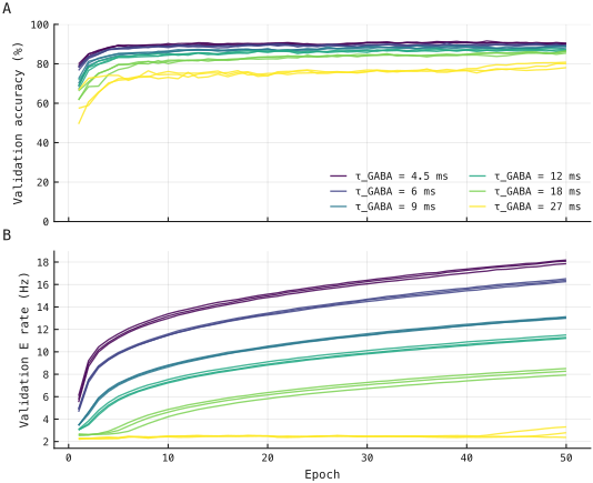
Figure 1: (A) Reused validation accuracy and (B) excitatory rate, one line per trained network across 50 epochs. Subsequent test measurements used final-epoch weights; accuracy convergence did not select the epoch.
Inhibitory-timescale spectra
Per-network interpolated frequencies spanned approximately 8–68 Hz across the inhibitory-decay sweep (Fig. 2).
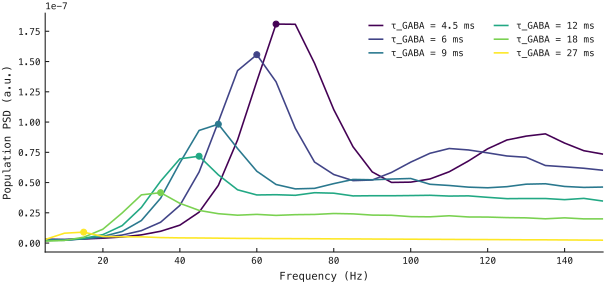
Figure 2: Population-E power spectral densities (PSDs), averaged across trials and then seeds at each inhibitory decay time. Dots mark binned peaks of these displayed means.
Inhibitory-timescale rasters
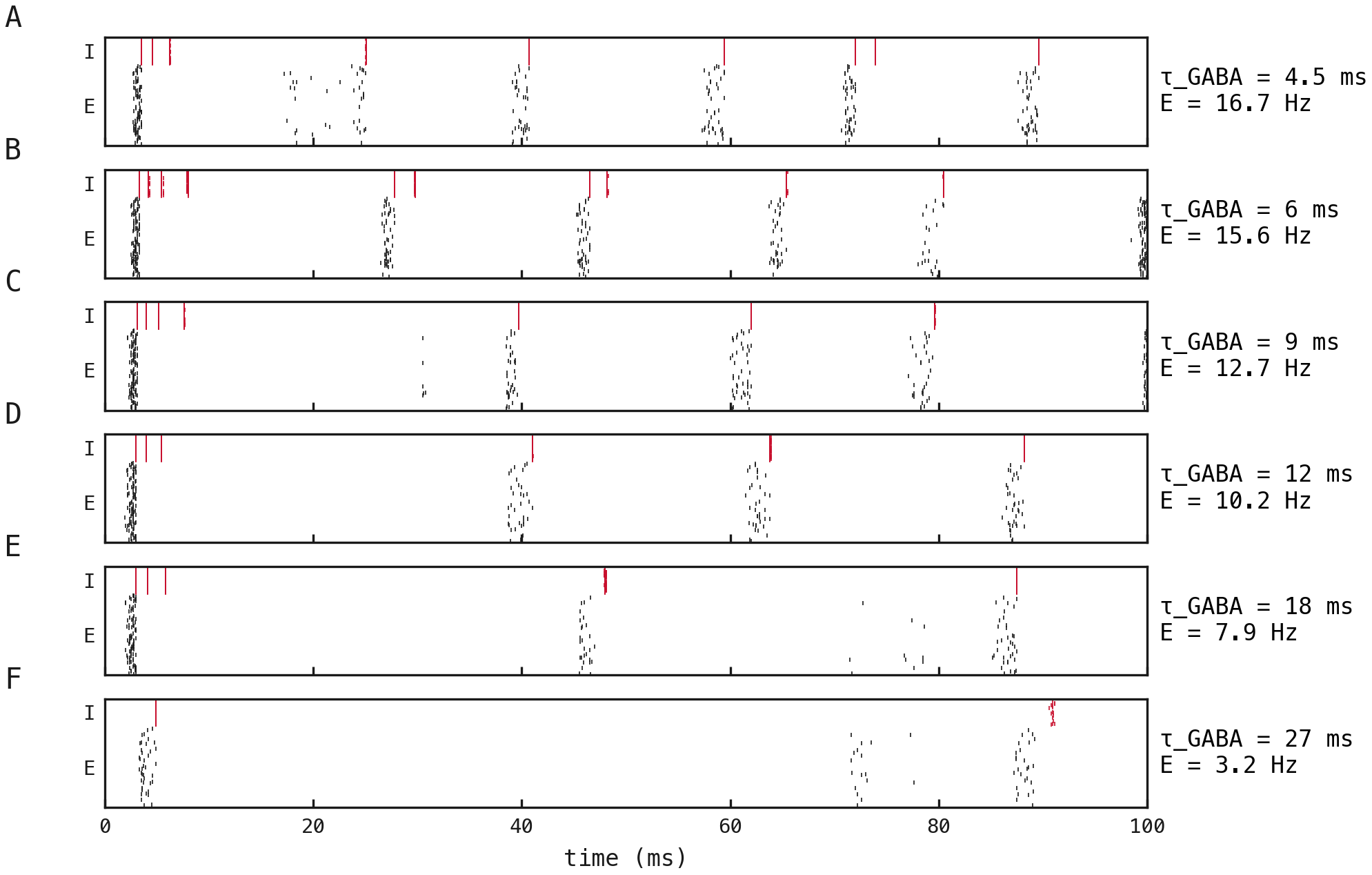
Figure 3: The same illustrative MNIST image at inhibitory decay times (A–F) 4.5, 6, 9, 12, 18 and 27 ms, respectively, using seed 42. Each panel shows 200 excitatory and 64 inhibitory neurons during the first 100 ms; displayed rates use the full populations and 200 ms trial. These probes illustrate timing, not the population frequency estimate.
Rate and accuracy versus frequency
Individual network rates spanned 2.3–18.4 Hz and accuracies 81–92% across the six inhibitory-decay conditions (Fig. 4).
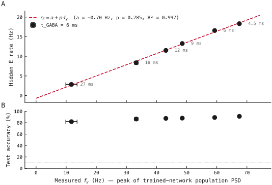
Figure 4: (A) Final-epoch excitatory rate and (B) test accuracy against gamma frequency. Each point is a mean over three seeds; error bars show ±1 standard error. The affine line fits six condition means.
Alternative rate-frequency fits
| fit | intercept (Hz) | slope (Hz/Hz) | |
| affine | -0.7 | 0.285 | 0.997 |
| through origin | 0 | 0.271 | 0.995 |
Table 1: Both least-squares fits used the same six condition means and centred total sum of squares. The origin-constrained fit tests how much the association depends on a free intercept.
Methods
We compared final-epoch dynamics across matched networks trained at different inhibitory decay times, keeping the evaluation data fixed.
-
Reuse matched trained networks. Six inhibitory GABA decay constants, ms, and seeds 42–44 defined 18 PING networks. Training used 6,300 MNIST training images and 700 held-out validation images, 50 epochs of AdamW with zero weight decay, learning rate , batches of 256, a time-averaged membrane-potential readout and no spike budget. Only inhibitory decay varied between conditions; simulation used 0.1 ms timesteps and 200 ms trials. We reused final-epoch weights to measure endpoint dynamics, without retraining or selecting weights by test performance.
-
Measure fixed-trial responses. Each network received the same fixed subset of 1000 images from the official MNIST test partition. We measured classification accuracy, mean excitatory spikes per neuron per second, and each trial’s population-E trace over the full 200 ms. The illustrative raster used image index 0 and seed 42; a fixed random seed of 0 selected displayed neurons without replacement.
-
Estimate rhythm frequency. We demeaned each trial’s trace and used a Welch density estimate with one full-trial Hann window [1], then averaged PSDs across trials. The largest peak between 5 and 150 Hz defined the candidate gamma frequency; its neighbouring linear-power values gave
(1)Here is the interpolated spectral-peak frequency, the peak-bin frequency, and Hz the bin spacing; , and are PSD values immediately below, at and above that bin. Because the peak search is restricted to the defined gamma band, the reported estimator is . We clamped the correction to half a bin, using zero offset for zero curvature or a spectrum endpoint. Interpolation reduces bin quantisation but can remain biased [2]. Per-trial peak distributions were diagnostics; their medians did not enter the fit.
-
Fit the rate–frequency relation. We averaged each network’s frequency and excitatory rate over the three seeds, then fitted the six condition points with equal weight by least squares:
(2)Here is mean excitatory firing rate in hertz, is the affine intercept in hertz, and and are dimensionless fitted slopes. Both fits report , the coefficient of determination using centred total sum of squares; error bars are sample standard deviations divided by .
-
Display matched endpoint evidence. We displayed the retained frequency, rate and accuracy comparisons across inhibitory decay times, preserving seed-level values and across-seed summaries.
Supplementary details
Appendix: Cycle-participation model
If a participation fraction of excitatory neurons emits exactly one spike during each cycle of duration , its cyclic per-neuron rate is . Adding a frequency-independent contribution gives
This is a proposed interpretation of the affine form, conditional on stable participation. Neurons nearest threshold when inhibition drops could contribute one spike while others recover; long inhibitory decay could instead sustain tonic inhibition and leave a feedforward contribution. Neither mechanism is established by the fit alone. In particular, an extrapolated intercept need not be a physical baseline, and a negative intercept cannot represent a nonnegative background firing rate.
Dataset
Figures use the recorded presentation selections and their same-experiment inputs. The table includes completed run history; the presentation used by this report is emphasized. Dates are run creation times in UTC; durations cover each stage separately, and sizes cover its exported files. For imported runs, durations and execution locations refer to the recorded producing execution.
Upstream: exp022 — Training Runs
Downstream: exp046 — One Spike per Gamma Cycle, exp110 — Manuscript
| Run | Date | Duration | Size | Ran on |
|---|---|---|---|---|
| exp041-r005-present | 2s | 572.7 KB | Local | |
| exp041-r002-analyse | 3s | 1.8 MB | Local | |
| exp041-r001-compute | — | 7.7 MB | Unknown |
References
-
P. D. Welch. “The use of the fast Fourier transform for the estimation of power spectra: A method based on time averaging over short, modified periodograms.” IEEE Transactions on Audio and Electroacoustics 15(2), 70–73 (1967). doi:10.1109/TAU.1967.1161901
-
J. O. Smith III. Spectral Audio Signal Processing. W3K Publishing (2011), “Quadratic Interpolation of Spectral Peaks” and “Bias of Parabolic Peak Interpolation.”