Training Recurrent Weights Weakens PING Rhythmicity
Trainable recurrent conductances produced lower reference-image rhythmicity and higher excitatory firing than the frozen PING control; outcomes depended on initialization.
Abstract
We asked whether surrogate-gradient training preserves PING rhythmicity when recurrent excitatory–inhibitory conductances can change. We compared trainable recurrent loops across initializations with a control whose recurrent PING weights remained frozen. Recurrent training weakened rhythmicity early and did not recover the rhythmic control, while activity and accuracy changed by condition. This constrains these learning recipes, but does not show that recurrent learning must always destroy gamma or that the compared conditions are accuracy-equivalent.
Results
E→I pruning accompanies low contrast
In all three networks in each condition, training from standard and 10%-standard recurrence drove most E→I weights to zero, while most I→E weights remained positive and their mean across all entries grew. Both conditions ended with lower reference-image contrast and higher E rates than frozen recurrence. Zero-initialized recurrence remained zero (Fig. 1). This pattern across three training replicates per condition remains descriptive: it does not isolate pruning as the cause of reduced contrast or establish equivalent accuracy.
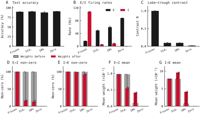
Figure 1: Final checkpoints: (A) official-test accuracy, (B) per-neuron E/I firing rates over the same 1000 test images and (C) unsmoothed reference-image contrast . Bars and error bars in A–C show means ±1 standard error of the mean (SEM) across three independently trained networks (sample standard deviation divided by ). In B, black denotes E and red I. Frozen denotes fixed standard recurrence; Std., 10% and Zero denote trainable recurrence initialized at standard, 10%-standard and zero weights. (D, E) Positive-weight fractions for E→I and I→E; (F, G) corresponding per-edge means including zeros, in model conductance units scaled by . For each direction, condition and time point, weight statistics pool 786,432 entries from three equal-sized matrices, giving each network equal weight. Wide grey bars show initialization and narrow red bars show epoch 50. Error bars show ±1 SEM across the three per-network statistics, calculated separately before and after training; they do not describe uncertainty in the paired change. Individual weights are not independent training replicates. Black arrows connect pooled values before and after when the relative change is at least 5%; this is a display threshold, not a statistical-significance test.
Rhythmicity starts low
The unsmoothed trainable contrast averaged 0.05 after epoch 1 and ended at 0.018–0.111. Because there is no epoch-0 observation, these histories cannot resolve the intervening transition (Fig. 2).
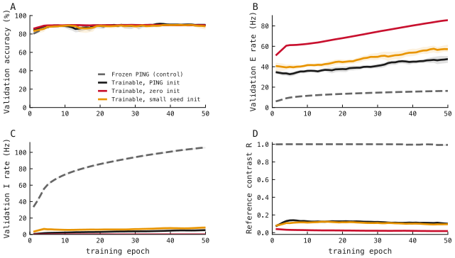
Figure 2: Recorded histories: (A) validation accuracy, (B) E rate, (C) I rate and (D) contrast from a fixed reference-image diagnostic. Lines show three-seed means; shading spans seed minima and maxima. Each series is smoothed with a five-epoch edge-padded moving average, not a confidence interval.
Methods
We reused networks from the exp022 — Training Runs (legacy) and reanalysed recorded observations. No new training or simulation was performed.
-
Compare recurrent trainability. Twelve conductance-based leaky-integrate-and-fire classifiers had 784 Poisson input channels, 1,024 excitatory (E), 256 inhibitory (I) and 10 output neurons. With three training replicates per condition, we compared frozen canonical recurrence with trainable canonical, zero and 10%-canonical E→I/I→E conductances; E→E and I→I coupling stayed zero. Canonical initializer means were and , respectively, with standard deviations one tenth of each mean and negative draws clamped to zero.
-
Train on a held-out split. The 7,000-image subset contained 6,300 optimizer-training and 700 validation images from the official MNIST training partition. Input and readout weights trained for 50 epochs with AdamW, learning rate , zero weight decay, batch size 256, surrogate slope 1, voltage-gradient damping 1,000, gradient-norm clipping at 1 and no firing-rate penalty. Class scores were mean pre-reset output voltages; each 200 ms presentation used 0.1 ms steps and pixel-dependent input rates up to 25 Hz.
-
Constrain conductance signs. Trainable recurrent magnitudes were projected onto the non-negative cone after each optimizer step. Inhibition arose through , where is inhibitory conductance, mV its reversal potential, and membrane voltage: a positive I→E weight need not become negative to inhibit. Input zeros remained trainable and could regrow.
-
Evaluate final networks. All endpoint tests and weight comparisons used epoch 50, not validation-selected weights. Accuracy and whole-population mean E/I rates used the same 1000 official-test images per network; per-epoch validation metrics averaged three fixed Poisson encoding draws. For endpoint spectra, demeaned nonconstant E-population traces received full-trial Welch density estimation; the mean spectrum’s largest bin within 5–150 Hz defined the selected peak, without interpolation.
-
Measure temporal contrast. After each epoch, the same fixed reference digit’s Poisson spike realization elicited a diagnostic response. E-population counts were binned at 1 ms; their autocorrelation was normalized by lag overlap and squared mean count, over 0–100 ms, then smoothed with weights after replacing the zero-lag entry by its neighbour:
(1)Here is dimensionless contrast, the first local trough from lag 2 ms onward, and the preceding positive-lag maximum of the smoothed autocorrelogram. We reused the recorded scalar; it is neither a test-population rhythm estimate nor a calibrated probability of PING.
-
Summarize recurrent weights. We reanalysed the initial and epoch-50 E→I and I→E matrices. For each direction and condition, we calculated the strictly positive fraction and arithmetic mean including zeros, both per network and over the three pooled matrices. Equal matrix sizes gave each network equal weight. Separately at each time point, we calculated SEM as the sample standard deviation of the three network summaries divided by . The independently trained network was the unit of replication; jointly trained weights were not additional replicates. These descriptive summaries did not test the significance of training-induced changes.
-
Expose retained training evidence. We displayed retained validation, activity and temporal-contrast measurements with their distinct training-replicate and illustrative-probe roles.
Dataset
Figures use the recorded presentation selections and their same-experiment inputs. The table includes completed run history; the presentation used by this report is emphasized. Dates are run creation times in UTC; durations cover each stage separately, and sizes cover its exported files. For imported runs, durations and execution locations refer to the recorded producing execution.
Upstream: exp022 — Training Runs
Downstream: exp110 — Manuscript
| Run | Date | Duration | Size | Ran on |
|---|---|---|---|---|
| exp049-r015-present | 4s | 2.6 MB | Local | |
| exp049-r013-analyse | 3s | 442.4 KB | Local | |
| exp049-r001-compute | — | 43.6 MB | Unknown |