Spike-Count Classification in a Continuous Stream
A multi-seed study of spike-count classification across input rates and presentation durations.
Abstract
Input calibration in exp080 — Decoder Accuracy Improves with Input Rate motivated the rate range used to train a variable rate PING classifier in exp022 — Training Runs. We tested whether these networks could classify continuous digit streams while retaining hidden state. With image sequences matched across conditions, longer, stronger inputs improved accuracy. One network classified five successive digits correctly despite changing durations and rates. Weak inputs exposed silent and incorrect responses. Decisions required supplied digit boundaries, and the selected successful example does not estimate reliability.
Results
Continuous classification and accuracy
One frozen PING network correctly classified five successive digits with varying presentation durations and input rates (Fig. 1A–D). Hidden neuronal state continued between digits, while output state and counts reset at supplied boundaries. This example demonstrates capability, not reliability across arbitrary streams. We reused the first stream with five correct decisions from a predefined candidate sequence; the first candidate qualified.
At 25 Hz, increasing presentation duration from 25 to 200 ms raised mean accuracy from 75.2% to 90.3% (Fig. 1E–F). At 200 ms, increasing input rate from 0.5 to 25 Hz raised accuracy from 26.3% to 90.3%. These comparisons used the same ordered images; variation from spike encoding and the small, fixed image sample remains.
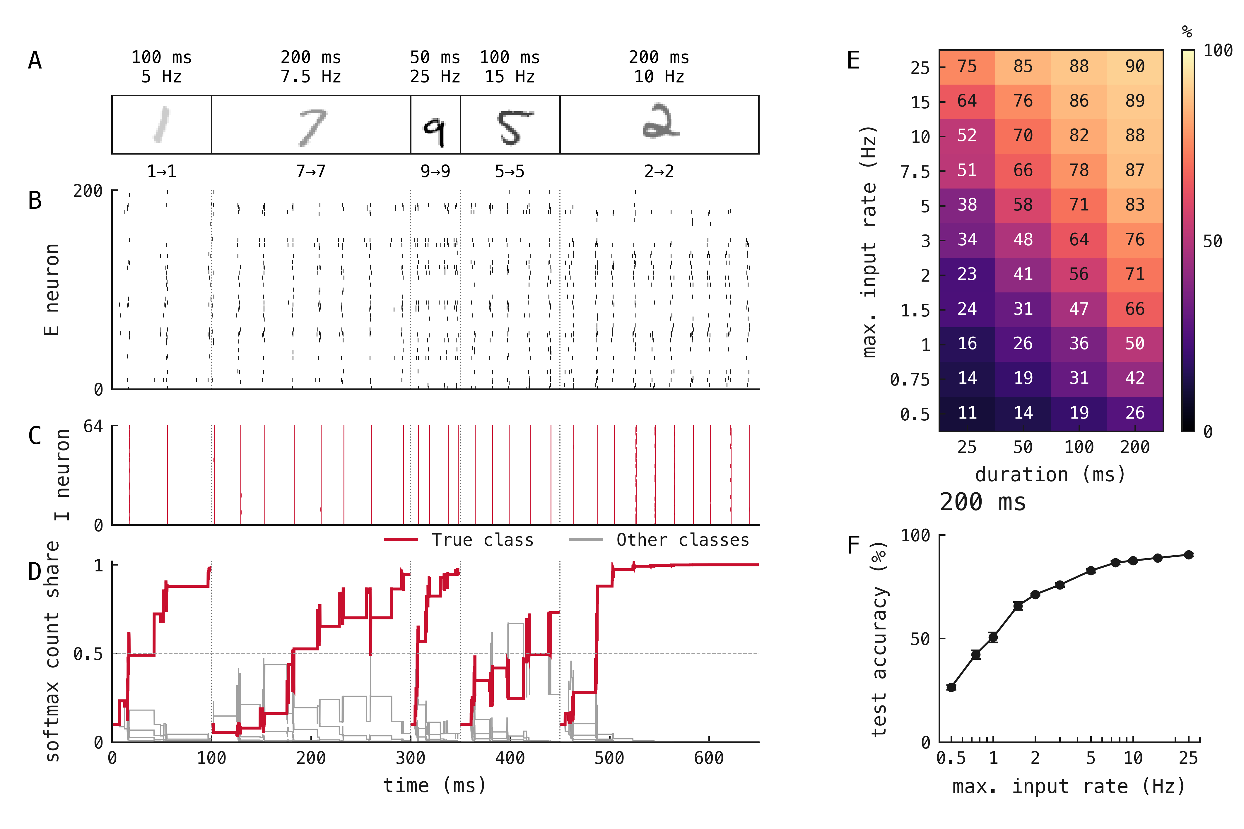
Figure 1: Seed-42 network presented with digits 1, 7, 9, 5 and 2. Each segment is labelled with its duration and maximum-pixel input rate. (A) Input thumbnails with true→predicted labels. (B) Spikes from the first 200 excitatory neurons; (C) spikes from the first 64 inhibitory neurons; (D) softmax-normalized output-count shares. Red traces identify the true classes. Panels A–D reuse the selected illustrative recording, independently of the quantitative evaluation in E–F. (E) Accuracy across presentation duration and maximum-pixel input rate; (F) the 200-ms rate–accuracy curve. Values are means across three independently trained networks, each evaluated on 200 digit presentations per condition. The same 40 ordered five-image streams were used for every network and condition, with separate encoding draws. E has no uncertainty intervals; F shows SEM across networks.
Spike counts identify the digit
By the presentation’s end, the true class, digit 4, had accumulated the largest output-spike count (Fig. 2). Intermediate leaders did not determine the decision.
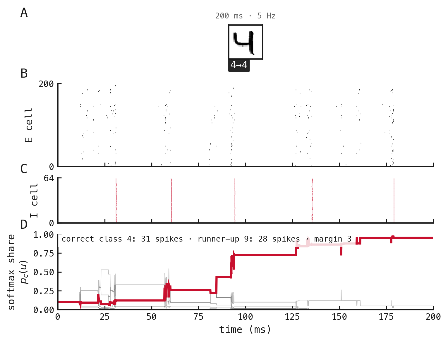
Figure 2: First correct digit in the seed-42 network’s matched 200-ms, 5-Hz stream. (A) Spikes from the first 200 excitatory neurons; (B) spikes from the first 64 inhibitory neurons; (C) softmax-normalized output-count shares. Red identifies the true class. These shares are not calibrated probabilities. The predicted digit is the class with the largest share at the presentation’s end.
Spikes change the displayed shares
Output counts stepped upward at spikes and remained constant between them (Fig. 3). Softmax normalization changed the displayed class shares at these increments; abrupt share changes need not reflect abrupt changes in the underlying network state.
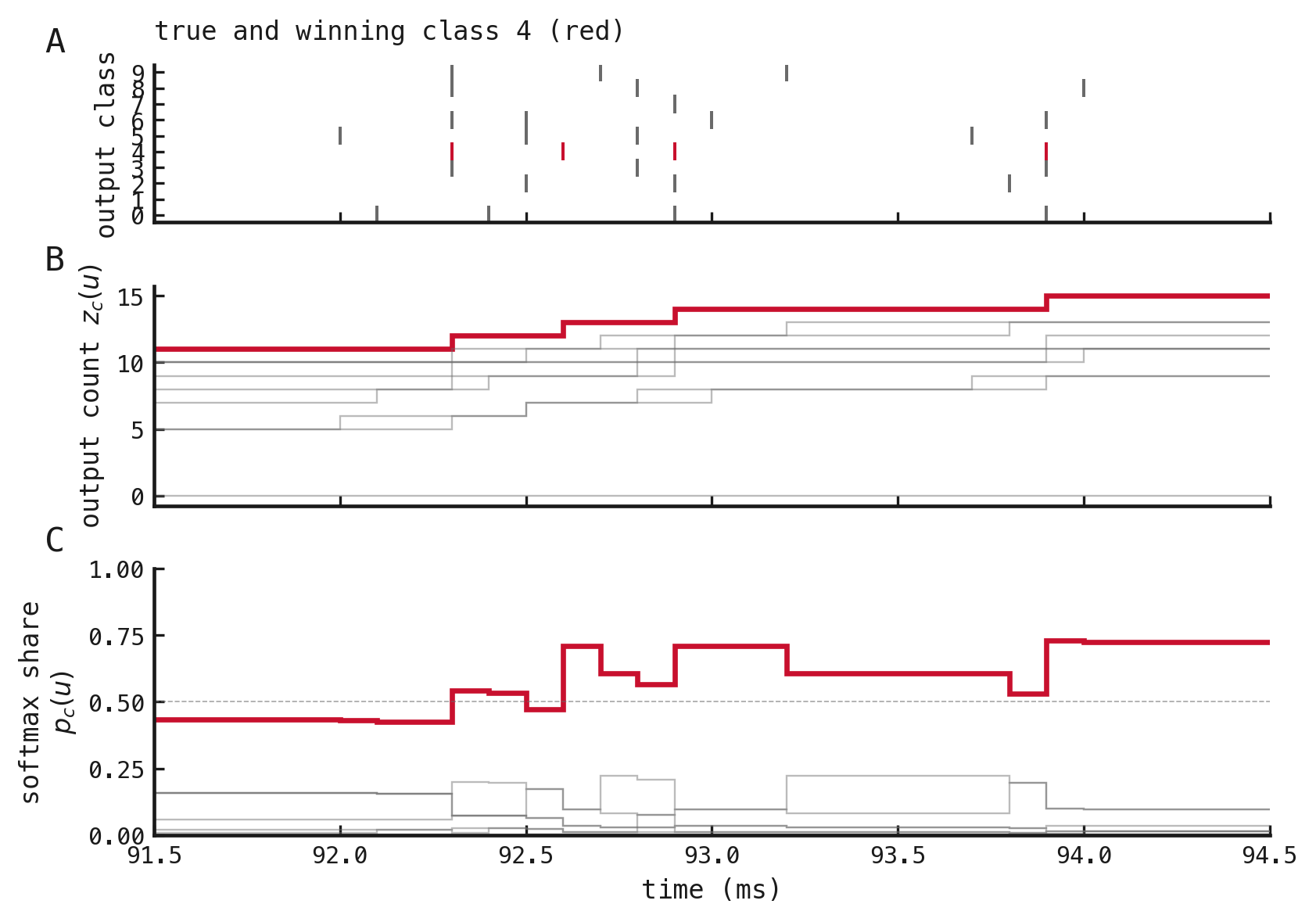
Figure 3: Post-hoc enlargement of 91.5–94.5 ms from the digit-4 presentation. (A) Output spikes; (B) cumulative class counts; (C) softmax-normalized count shares. Red identifies the true class.
Weak inputs expose failure modes
A stream with varying durations and input rates produced 3 correct decisions (Fig. 4). The 200-ms, 0.5-Hz presentation produced no output spikes, whereas the 100-ms, 2-Hz presentation was misclassified despite output activity.
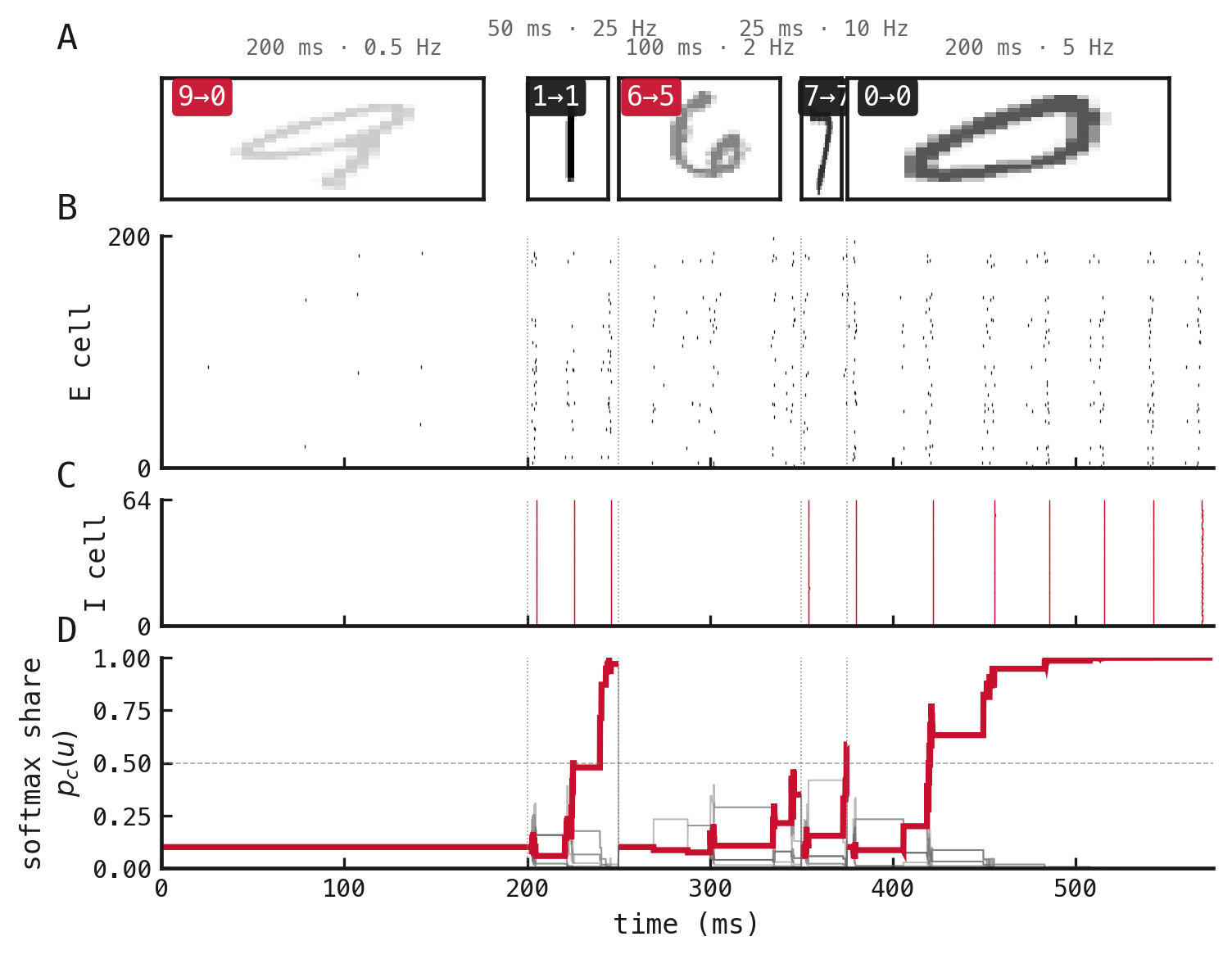
Figure 4: Seed-42 network under the duration–rate conditions labelled above each segment. (A) Input thumbnails; (B) excitatory spikes; (C) inhibitory spikes; (D) softmax-normalized output-count shares. Badges show true→predicted labels. Thumbnail opacity indicates relative input rate; population sampling matches Figure 1.
Methods
-
Input range and classifiers. The filtered-input calibration in exp080 — Decoder Accuracy Improves with Input Rate motivated the input-rate range. We reused three frozen networks, trained with seeds 42–44, from exp022 — Training Runs. Each contained 1,024 excitatory neurons, 256 inhibitory neurons and ten output leaky integrate-and-fire neurons, with learned input-to-excitatory and excitatory-to-output projections and fixed recurrent weights. Evaluation held all weights fixed; the revised sampling protocol did not require retraining.
-
Simulation and refractory periods. We used a 0.1-ms integration timestep. Hidden excitatory and inhibitory neurons remained at reset for 1.2 and 0.6 ms after a spike, respectively, corresponding to 12 and six timesteps. Output neurons had no refractory period. The repeated evaluation specified these physical durations explicitly, preserving the refractory holds used by the earlier fixed-timestep measurements.
-
Training and checkpoint selection. Training used 6,300 optimization images and 700 validation images for 50 epochs. Maximum-pixel input rates were sampled from 0.5, 0.75, 1, 1.5, 2, 3, 5, 7.5, 10, 15 and 25 Hz. After each epoch, we evaluated the network on three independently spike-encoded versions of the validation images. Mean validation cross-entropy was
(1)Here is the number of validation images, is the number of encoding draws, is the true class of image , and is its true-class softmax share for draw , defined below. We selected the epoch with the lowest . If epochs tied, we chose the one with higher validation accuracy, then the earlier epoch.
-
Evaluation streams. We repeated the quantitative evaluation using one prespecified bank of 40 five-image streams from the official 10,000-image MNIST test partition. Image sampling used seed 82000. Within each stream, we sampled five images uniformly without replacement and without class stratification; labels could repeat and images could recur across streams. Every network, duration and input rate used the same ordered image indices, so both image identity and preceding-image order were paired across conditions. We tested all eleven training rates at 25, 50, 100 and 200 ms (Fig. 1E–F). Each duration–rate–network condition contained 40 five-digit streams, giving 200 decisions. The 132 network–duration–rate conditions therefore yielded 26,400 decisions, not 26,400 independently sampled images. Duration and rate were constant within each quantitative stream. Batches contained five streams with separate neuronal states.
-
Earlier evaluation and pairing. The earlier evaluation sampled images separately by condition. Its seed formula mapped 44 duration–rate combinations onto only 34 image-sampling seeds per network: ten pairs shared identical streams while the other conditions remained unpaired. The current quantitative results replace that mixed design with a common image bank. Image selection and encoding seeds both changed; differences from the earlier estimates cannot be attributed to image pairing alone. We reused the previously selected capability recording independently of this repeated grid evaluation.
-
Input encoding. Pixels generated independent Bernoulli spikes at 0.1-ms resolution. Spike probability was proportional to pixel intensity and the condition’s maximum-pixel input rate. Image selection and spike encoding used separate random generators. Each network–duration–rate–stream combination had a distinct encoding seed, giving 5,280 seeds across the quantitative grid. Each generator advanced across its stream’s five presentations. Pairing therefore matched images and their order, not realized input spike trains. Digits followed without gaps; segment labels give their durations and input rates (Fig. 1A and Fig. 4A).
-
State and decision boundaries. Each stream began with freshly initialized hidden and output states. Hidden neuronal and synaptic state then persisted between digits within that stream. Output-neuron state and spike counts reset at every supplied digit boundary. The readout accumulated evidence over the full presentation (Fig. 1B–D and Fig. 4B–D).
-
Spike-count classification. The cumulative score for class at timestep was
(2)where is the first timestep of the presentation and equals 1 when output neuron spikes at timestep , and 0 otherwise. The displayed class share was
where indexes the ten digit classes. These softmax shares are not calibrated probabilities.
At the final timestep , we predicted
(4)where is the predicted digit: the class with the greatest final cumulative count, equivalently the largest final displayed share (Fig. 2C). Ties selected the lowest class index, including class 0 when all outputs were silent.
-
Performance summaries. We calculated accuracy for each duration–rate–network condition and summarized network-level measurements as means and SEM across three training replicates (Fig. 1E–F). Accuracy included silent presentations and all other decisions. SEM was sample SD divided by the square root of three; it summarizes observed variation across networks and their encoding draws, not uncertainty across independent image banks. The 200-ms curve reuses the corresponding heatmap evaluations. One shared image bank and one encoding draw per network, condition and stream do not separately estimate image-sampling, encoding and training variability.
-
Capability example. We reused a seed-42 recording selected with the predefined sequence of duration–rate pairs: (100 ms, 5 Hz), (200 ms, 7.5 Hz), (50 ms, 25 Hz), (100 ms, 15 Hz) and (200 ms, 10 Hz). We fixed candidate order and digit-sampling and encoding seeds before inference. Fig. 1 uses the first candidate achieving five correct decisions. This search used five distinct digit classes per candidate, unlike the quantitative image sampling, which allowed repeated labels. The first candidate, with image-selection seed 820000 and encoding seed 830000, qualified. It was not drawn from the quantitative image bank.
-
Failure example. We reused a separately specified seed-42 stream with pairs (200 ms, 0.5 Hz), (50 ms, 25 Hz), (100 ms, 2 Hz), (25 ms, 10 Hz) and (200 ms, 5 Hz). This example was not selected through the capability search (Fig. 4).
-
Readout close-up. We selected the first correct digit from a separate 200-ms, 5-Hz stream (Fig. 2) and enlarged its 91.5–94.5-ms interval post hoc (Fig. 3). Equations Equation 2 and Equation 3 define the displayed counts and shares.
-
Scope of inference. We evaluated classification with known boundaries and continuing hidden state, without testing autonomous segmentation, a hidden-state-reset control, or gamma activity’s causal contribution to recognition. Presentation and readout windows changed together, so the duration comparison does not separate extra sensory exposure from extra integration time. The selected success and separately specified failure stream are illustrations, not estimates of the frequency of such outcomes.
Dataset
Figures use the recorded presentation selections and their same-experiment inputs. The table includes completed run history; the presentation used by this report is emphasized. Dates are run creation times in UTC; durations cover each stage separately, and sizes cover its exported files. For imported runs, durations and execution locations refer to the recorded producing execution.
Upstream: exp022 — Training Runs
Downstream: exp110 — Manuscript
| Run | Date | Duration | Size | Ran on |
|---|---|---|---|---|
| exp082-r033-present | 3s | 1.5 MB | Local | |
| exp082-r032-analyse | 2s | 174.2 KB | Local | |
| exp082-r031-compute | — | 686.6 KB | Unknown |