Mean-field Frequency Coupling

Unwrapped relative phase before and after reciprocal coupling in delayed mean-field circuits.

Experiment

exp153

Created

25 Oct 26

Updated

25 Oct 26

Collections

Paper Inspired
Experiments

Report

312 words1 figure3 runs

Abstract

Reciprocal coupling arrests phase drift between two delayed mean-field circuits derived from exp133. Circuit B’s rate relaxation is 20% faster, creating a visible intrinsic mismatch.

Results

Relative phase falls by 1.7 cycles before coupling at 500 ms, then settles near −2 cycles.

The uncoupled frequencies are 25.25/28.60 Hz; coupling brings both to about 23.28 Hz, with residual drift 0.0002 cycles/s.

This demonstrates entrainment over the measured window for one initial history.

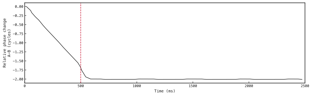
Relative phase drifts before coupling at 500 ms, then plateaus. — **Figure 1.**
Unwrapped A-minus-B E-rate phase, zeroed at the first common observed sample. Red dashed line: 0.08 µS coupling enabled at 500 ms. Phase is interpolated between peaks on a 0.5 ms grid without smoothing or extrapolation. Frequencies and drift use 800–2,500 ms; the uncoupled control continues drifting.

Methods

SNNLab reduces the imported network to four rates and ten conductance filters, with 0.1 ms internal and 2 ms cross-circuit delays.

E/I relaxation times are 20/5 ms in A and 16/4 ms in B.

The boxes show all native exported dynamical equations with compact display notation, followed by the current definitions.

Circuits are superscripts A/B; E/I denote excitatory/inhibitory populations. For a pathway such as AE → BI, the first pair identifies its source and the second its target; xA/xB denote external inputs. All 14 dynamical equations and their current definitions are shown below.

Population-rate functions

\begin{aligned}\tau_{r,E}^{A}\,\dot{r_{E}^{A}} &= - r_{E}^{A} + \Phi_{E}^{A}{\left(I_{E}^{A} \right)} \\ \tau_{r,I}^{A}\,\dot{r_{I}^{A}} &= - r_{I}^{A} + \Phi_{I}^{A}{\left(I_{I}^{A} \right)} \\ \tau_{r,E}^{B}\,\dot{r_{E}^{B}} &= - r_{E}^{B} + \Phi_{E}^{B}{\left(I_{E}^{B} \right)} \\ \tau_{r,I}^{B}\,\dot{r_{I}^{B}} &= - r_{I}^{B} + \Phi_{I}^{B}{\left(I_{I}^{B} \right)}\end{aligned}

Conductance-filter functions

\begin{aligned}\dot{g_{AE\to AI}} &= - \frac{g_{AE\to AI}}{\tau_{AE\to AI}} + \frac{C_{AE\to AI} r_{E}^{A}(t-0.1) a_{AE\to AI}}{1000} \\ \dot{g_{AE\to BE}} &= - \frac{g_{AE\to BE}}{\tau_{AE\to BE}} + \frac{C_{AE\to BE} r_{E}^{A}(t-2) a_{AE\to BE}}{1000} \\ \dot{g_{AE\to BI}} &= - \frac{g_{AE\to BI}}{\tau_{AE\to BI}} + \frac{C_{AE\to BI} r_{E}^{A}(t-2) a_{AE\to BI}}{1000} \\ \dot{g_{AI\to AE}} &= - \frac{g_{AI\to AE}}{\tau_{AI\to AE}} + \frac{C_{AI\to AE} r_{I}^{A}(t-0.1) a_{AI\to AE}}{1000} \\ \dot{g_{xA\to AE}} &= - \frac{g_{xA\to AE}}{\tau_{xA\to AE}} + \frac{C_{xA\to AE} a_{xA\to AE} \nu^{A}}{1000} \\ \dot{g_{BE\to BI}} &= - \frac{g_{BE\to BI}}{\tau_{BE\to BI}} + \frac{C_{BE\to BI} r_{E}^{B}(t-0.1) a_{BE\to BI}}{1000} \\ \dot{g_{BE\to AE}} &= - \frac{g_{BE\to AE}}{\tau_{BE\to AE}} + \frac{C_{BE\to AE} r_{E}^{B}(t-2) a_{BE\to AE}}{1000} \\ \dot{g_{BE\to AI}} &= - \frac{g_{BE\to AI}}{\tau_{BE\to AI}} + \frac{C_{BE\to AI} r_{E}^{B}(t-2) a_{BE\to AI}}{1000} \\ \dot{g_{BI\to BE}} &= - \frac{g_{BI\to BE}}{\tau_{BI\to BE}} + \frac{C_{BI\to BE} r_{I}^{B}(t-0.1) a_{BI\to BE}}{1000} \\ \dot{g_{xB\to BE}} &= - \frac{g_{xB\to BE}}{\tau_{xB\to BE}} + \frac{C_{xB\to BE} a_{xB\to BE} \nu^{B}}{1000}\end{aligned}

Effective currents

\begin{aligned}I_{E}^{A} &= I_{\mathrm{ext},E}^{A} + \Delta V_{e,E}^{A} \left(g_{xA\to AE} + g_{BE\to AE}\right) - \Delta V_{i,E}^{A} g_{AI\to AE} \\ I_{I}^{A} &= I_{\mathrm{ext},I}^{A} + \Delta V_{e,I}^{A} \left(g_{AE\to AI} + g_{BE\to AI}\right) \\ I_{E}^{B} &= I_{\mathrm{ext},E}^{B} + \Delta V_{e,E}^{B} \left(g_{AE\to BE} + g_{xB\to BE}\right) - \Delta V_{i,E}^{B} g_{BI\to BE} \\ I_{I}^{B} &= I_{\mathrm{ext},I}^{B} + \Delta V_{e,I}^{B} \left(g_{AE\to BI} + g_{BE\to BI}\right)\end{aligned}

Time is in ms; dots denote time derivatives. Symbols: r, rate (Hz);g, conductance (µS); I, current (nA); τ, relaxation or decay time (ms); C, mean incoming weight (µS); a, dimensionless delivery-time gain; ΔV, fixed driving force (mV); Φ, noisy-LIF current-to-rate function; ν, external input rate (Hz). Subscript ext denotes applied current; e/i denote excitatory/inhibitory driving forces. Cross-circuit gains switch from zero to one at 500 ms; other gains are constant. The factor 1/1000 converts Hz to events per ms.

Both trajectories use constant prehistory, initial rates of 1 Hz and zero conductances. Integration uses DOP853 with maximum step 0.1 ms and tolerances $10^{-8}$ relative/ $10^{-10}$ absolute. Phase statistics require sustained regular rhythms; locking thresholds and all parameters are in the appendix. The unfitted closure omits input covariance, finite-population fluctuations and shunting.

Network

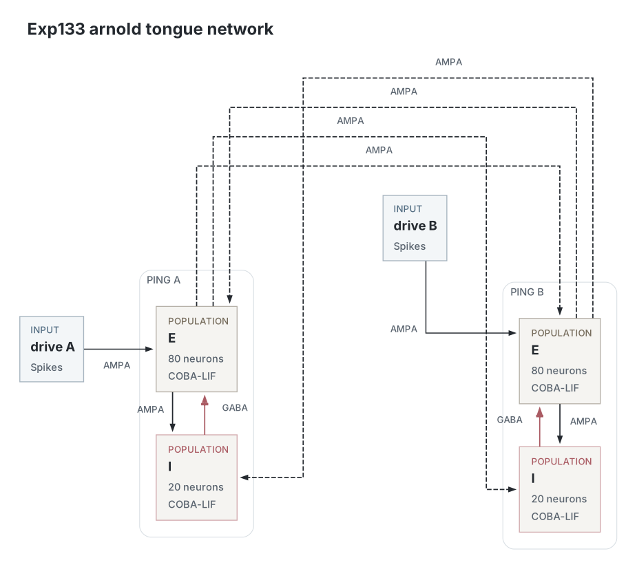
Saved exp133 paired PING circuits, with reciprocal excitation from each E population to the other circuit's E and I populations. — **Figure 2.**
Circuit diagram generated from the authenticated source bundle used in the reduction. Two 80-E/20-I circuits retain their separate external source pools. The mean-field model replaces each population by one rate and each incoming pathway by a conductance filter; neuron counts define imported weight sums, rather than the number of dynamical rate variables.

Parameters

The retained native snapshot describes the imported spiking reference, not a spiking simulation performed by exp153. Numerical integration settings and closure choices come from the selected exp153 compute record. Reference cross-circuit sums are multiplied by nominal coupling divided by 0.12 µS; the uncoupled control sets them to zero. Input gain is already present in the effective native input matrices. There is no additional factor of 9.2 and no resampling of connectivity.

Parameter	Value
Network and imported neurons
PING_A_E neurons	80
PING_A_E capacitance / leak (nF / µS)	1 / 0.05
PING_A_E rest / reset / threshold (mV)	-65 / -65 / -50
PING_A_E refractory (ms)	3
PING_A_I neurons	20
PING_A_I capacitance / leak (nF / µS)	0.5 / 0.1
PING_A_I rest / reset / threshold (mV)	-65 / -65 / -50
PING_A_I refractory (ms)	1.5
PING_B_E neurons	80
PING_B_E capacitance / leak (nF / µS)	1 / 0.05
PING_B_E rest / reset / threshold (mV)	-65 / -65 / -50
PING_B_E refractory (ms)	3
PING_B_I neurons	20
PING_B_I capacitance / leak (nF / µS)	0.5 / 0.1
PING_B_I rest / reset / threshold (mV)	-65 / -65 / -50
PING_B_I refractory (ms)	1.5
Synapses and derived weights
PING_A_E_to_I decay / delay (ms)	1 / 0.1
PING_A_E_to_I reference mean incoming weight (µS)	0.4985915
PING_A_E_to_PING_B_E_K_EE decay / delay (ms)	2 / 2
PING_A_E_to_PING_B_E_K_EE reference mean incoming weight (µS)	0.1200000
PING_A_E_to_PING_B_I_K_EI decay / delay (ms)	2 / 2
PING_A_E_to_PING_B_I_K_EI reference mean incoming weight (µS)	0.1200000
PING_A_I_to_E decay / delay (ms)	9 / 0.1
PING_A_I_to_E reference mean incoming weight (µS)	1.004179
PING_A_input_to_E decay / delay (ms)	2 / 0
PING_A_input_to_E reference mean incoming weight (µS)	1.842201
PING_B_E_to_I decay / delay (ms)	1 / 0.1
PING_B_E_to_I reference mean incoming weight (µS)	0.4991069
PING_B_E_to_PING_A_E_K_EE decay / delay (ms)	2 / 2
PING_B_E_to_PING_A_E_K_EE reference mean incoming weight (µS)	0.1200000
PING_B_E_to_PING_A_I_K_EI decay / delay (ms)	2 / 2
PING_B_E_to_PING_A_I_K_EI reference mean incoming weight (µS)	0.1200000
PING_B_I_to_E decay / delay (ms)	9 / 0.1
PING_B_I_to_E reference mean incoming weight (µS)	0.9981220
PING_B_input_to_E decay / delay (ms)	2 / 0
PING_B_input_to_E reference mean incoming weight (µS)	1.834603
Closure choices and numerical calculation
Source network seed	85
Voltage-noise scale (mV)	4
A E / I rate relaxation (ms)	20 / 5
B E / I rate relaxation (ms)	16 / 4
B relaxation multiplier	0.8
Gain quadrature nodes	48
Driving force / external filtering	Fixed resting / dynamic
Transmission delays	explicit
Initial rates / conductances (Hz / µS)	1 / 0
Prehistory	constant
Duration / observation interval (ms)	2500 / 0.5
Integrator / maximum step (ms)	DOP853 / 0.1
Relative / absolute tolerance	1e-8 / 1e-10
Input mean (Hz/source)	25
Input difference (Hz/source)	10
Uncoupled / onset coupling (µS)	0 / 0.08
Condition count	2
Coupling-onset time (ms)	500
Analysis
Sustained-rhythm windows (ms)	800–1600; 1600–2500
Absolute / relative amplitude floor (Hz / fraction)	0.5 / 0.01
Minimum late / early amplitude ratio	0.5
Minimum peaks / maximum interval CV	15 / 0.2
Frequency matching requirement	None; measured rhythm frequency
Settled phase-window start (ms)	800
Maximum drift (cycles/s)	0.25
Minimum concentration / maximum span (cycles)	0.95 / 1

The native mean-field model document records symbolic equations and delayed dependencies. Each trajectory retains its constant history, actual parameters, delivery-time controls and solver settings. These finite-time measurements do not constitute a delayed stability proof. See the mean-field note for the stationary-gain closure and its limitations.

Dataset

Upstream: exp133 — Lowet (2015): Coupled Rhythms

Downstream: —

Run	Date	Duration	Size	Evidence	Storage	Ran on	Verification
exp153-r019-present	25 Oct 2026, 18:46	<1s	594 KB	Current	R2	Local	Local: absent; R2: catalog-verified
exp153-r017-analyse	25 Oct 2026, 18:44	<1s	366.7 KB	Current	R2	Local	Local: absent; R2: catalog-verified
exp153-r016-compute	25 Oct 2026, 18:43	15s	4.3 MB	Current	R2	Local	Local: absent; R2: catalog-verified
exp133-r039-present	16 Oct 2026, 12:52	1s	497.5 KB	Current	R2	Local	Local: absent; R2: catalog-verified
exp133-r038-analyse	16 Oct 2026, 12:52	1s	124.2 KB	Current	R2	Local	Local: absent; R2: catalog-verified
exp133-r037-compute	16 Oct 2026, 12:52	6s	2 MB	Current	R2	Local	Local: absent; R2: catalog-verified
exp133-r029-analyse	16 Oct 2026, 12:16	3s	107.6 KB	Current	R2	Local	Local: absent; R2: catalog-verified
exp133-r028-compute	16 Oct 2026, 12:10	4m 53s	31.7 MB	Current	R2	Local	Local: absent; R2: catalog-verified
exp133-r025-compute	16 Oct 2026, 11:51	4m 18s	11.5 MB	Current	R2	Local	Local: absent; R2: catalog-verified