Lowet (2015): Coupled Rhythms
A gamma phase-locking map and coupling-onset demonstration inspired by Lowet et al. (2015).
Abstract
We tested whether reciprocal excitation synchronizes two conductance-based gamma circuits across 143 combinations of input imbalance and coupling strength, with 1,024 input channels per circuit and mean input 25 Hz per channel. Thirteen settings met finite-time locking criteria; maximum valid phase-locking value (PLV) was 0.990. A selected coupling-onset diagnostic also reached PLV 0.990 over 800–1,500 ms. These results describe one network initialization and paired input realization, without testing repeatability across seeds or lasting locking.
Results
Reciprocal coupling and phase locking
Inspired by Lowet et al. (2015), we tested when two gamma rhythms hold a steady phase difference. Across 143 settings, 141 had valid rhythms and 13 met all finite-time locking criteria; maximum valid PLV was 0.99 (Fig. 1). PLV measures consistency of relative phase, from zero to one; a value near one need not mean zero phase difference. This sampled map describes one realization and does not establish a continuous locking boundary or robustness across seeds.
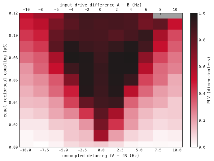
Each rectangle is one sampled setting. Bottom: uncoupled A-minus-B frequency difference (Hz); top: A-minus-B input-rate difference (Hz per channel). Vertical axis: equal nominal total coupling per pathway (μS). White–red–black indicates increasing PLV; gray marks invalid rhythms. Values use common phase-valid samples within 800–5,000 ms. Cell edges delimit sampled settings, not inferred boundaries.
Lowet et al.’s published map provides a qualitative comparison (Fig. 2). Their conductance-density coupling, Hodgkin–Huxley neurons and signal-based phase estimate differ from our conductance-LIF model and excitatory-volley phase, so the displays do not provide a quantitative replication.
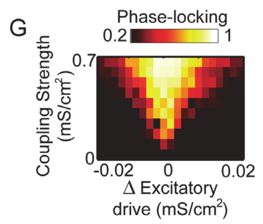
Crop of Lowet et al. (2015), Fig. 2G. Brighter colors indicate stronger PLV. Axes show input-drive difference and coupling in mS/cm²; Fig. 1 uses measured frequency difference in Hz and coupling in μS. Original labels and colors retained. © 2015 Lowet et al., Creative Commons Attribution.
Switching on reciprocal coupling
We used the map’s −4 Hz input difference and 0.09 μS coupling, keeping its saved weights and connections in both directions. At 500 ms, we switched coupling on. S/R frequencies changed from 41.6/46 Hz to 45.7/45.7 Hz. Relative phase became nearly steady (Fig. 3); PLV was 0.99, fitted drift was 0.0077 cycles/s and phase span was 0.115 cycles over 800–1,500 ms.
This diagnostic reuses the selected map matrices and input realization; its spikes match that map trajectory over the displayed interval. It illustrates the onset of finite-time locking and is not an independent evaluation or evidence of lasting locking.
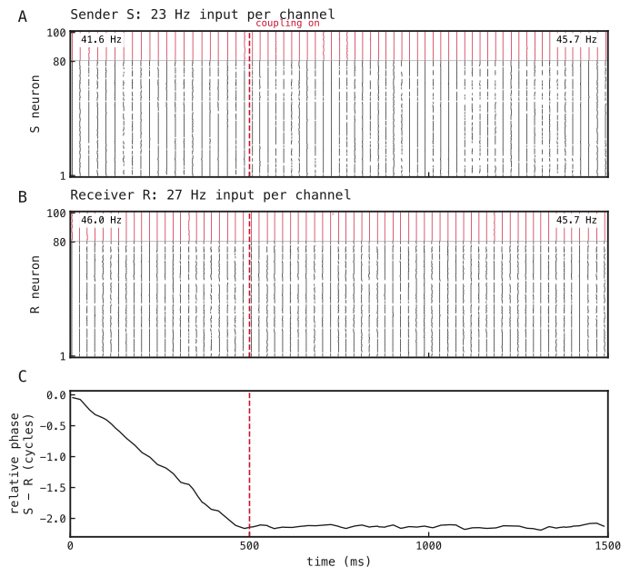
(A) Sender S and (B) receiver R spikes: excitatory neurons in black, inhibitory neurons in red. Input rates are 23/27 Hz per channel for S/R. Dashed lines mark coupling onset at 500 ms. Corner values give frequency over 0–500 ms and 1,000–1,500 ms. (C) Unwrapped S-minus-R phase difference in cycles, shown between detected excitatory volleys. Phase metrics use shared valid times within 800–1,500 ms.
Methods
-
Construct the paired circuits. Use the saved conductance-based leaky integrate-and-fire (conductance-LIF) networks in Fig. A1, with parameters in Table A1. Binary input spikes are drawn independently per channel and timestep, with probability equal to input rate times timestep in seconds. Split each original input afferent into eight channels with one-eighth weight, preserving summed input strength and recurrent matrices. No weights are trained.
-
Sweep reciprocal coupling (Fig. 1). Cross 11 input differences (−10 to +10 Hz per channel, step 2 Hz) with 13 coupling strengths (0–0.12 μS, step 0.01 μS). Mean input stays 25 Hz per channel. Copy a shared 500 ms uncoupled prefix into each coupling condition, then simulate to 5,000 ms without resetting state. Reuse inputs across coupling strengths and underlying random draws across input differences. Exclude 300 ms after coupling onset. The zero-coupling condition supplies measured frequency detuning. Batched settings are conditions, not replicates.
-
Measure relative phase (Figs. 1 and 3). Smooth excitatory population rate with a Gaussian of 1 ms standard deviation; detect peaks separated by at least 15 ms with prominence at least 10% of the maximum smoothed rate. Interpolate phase linearly between consecutive volleys, advancing by radians per interval; omit samples outside observed volleys. Compute
Here and are circuit phases in radians at shared valid sample , is the number of those samples, is the imaginary unit, and bars denote complex magnitude. Use S/R in place of A/B for Fig. 3. Estimate frequency as the reciprocal mean inter-volley interval, drift as the least-squares slope of unwrapped relative phase in cycles against seconds, and span as its maximum minus minimum. For the map, each rhythm needs at least 20 volleys, frequency 30–80 Hz and interval coefficient of variation (standard deviation divided by mean) ≤0.2; its uncoupled calibration must also pass. Valid pairs meet the diagnostic locking criteria when absolute drift <0.25 cycles/s, PLV >0.95 and span <1 cycle. These thresholds describe finite windows.
-
Inspect coupling onset (Fig. 3). Transfer the selected map’s input, local and both cross-network matrices with A→S and B→R, retaining the same inputs. Apply native step gain, zero before 500 ms and one thereafter, for a continuous 1,500 ms trajectory. Phase metrics use 100–500 ms before coupling and 800–1,500 ms after coupling. Raster frequencies use the first and last 500 ms; each window requires at least five volleys and the same frequency and interval-regularity checks. Retained-evidence checks compare transferred matrices, eight-afferent masks, scheduled gains and unchanged parameters; exact spike agreement with the map checks transfer consistency, not independent reproducibility.
Network diagrams
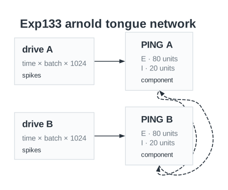
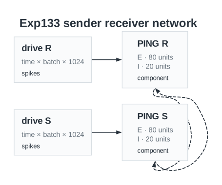
Saved circuit diagrams for (A) the coupling map and (B) the sender–receiver run. E and I denote excitatory and inhibitory populations. Arrows show local and reciprocal pathways. Labels show base input strengths before the request gain in Table A1.
Parameters
| Parameter | Coupling map | Onset diagnostic |
|---|---|---|
| Network | ||
| Neurons per circuit, E / I | 80 / 20 | 80 / 20 |
| Input channels per circuit | 1024 | 1024 |
| Neuron model | Conductance-LIF | Conductance-LIF |
| Reciprocal pathways | A E→B E/I and B E→A E/I | S E→R E/I and R E→S E/I |
| Neurons | ||
| Capacitance, E / I | 1 / 0.5 nF | 1 / 0.5 nF |
| Leak conductance, E / I | 0.05 / 0.1 µS | 0.05 / 0.1 µS |
| Passive time constant, E / I (derived) | 20 / 5 ms | 20 / 5 ms |
| Resting voltage, E / I | -65 / -65 mV | -65 / -65 mV |
| Reset voltage, E / I | -65 / -65 mV | -65 / -65 mV |
| Initial voltage, E / I | -65 / -65 mV | -65 / -65 mV |
| Spike threshold, E / I | -50 / -50 mV | -50 / -50 mV |
| Refractory period, E / I | 3 / 1.5 ms | 3 / 1.5 ms |
| Synapses and weights | ||
| Input→E base initializer mean / SD | 0.2 / 0.03 µS | 0.2 / 0.03 µS |
| Input→E request gain | 9.2 | 9.2 |
| Input→E nominal mean / SD after gain (derived) | 1.84 / 0.276 µS | 1.84 / 0.276 µS |
| E→I initializer mean / SD | 0.5 / 0.05 µS | 0.5 / 0.05 µS |
| I→E initializer mean / SD | 1 / 0.1 µS | 1 / 0.1 µS |
| Input→E synapse / decay | AMPA / 2 ms | AMPA / 2 ms |
| E→I synapse / decay | AMPA / 1 ms | AMPA / 1 ms |
| I→E synapse / decay | GABA / 9 ms | GABA / 9 ms |
| Local E→I / I→E delay | 0.1 / 0.1 ms | 0.1 / 0.1 ms |
| Cross-network nominal total per pathway | 0, 0.01, 0.02, 0.03, 0.04, 0.05, 0.06, 0.07, 0.08, 0.09, 0.1, 0.11, 0.12 µS | 0.09 µS |
| Cross-network fan-in (derived) / zero fraction | 8 / 0.9 | 8 / 0.9 |
| Cross-network zeroing / initializer SD | Exact fan-in / 0 µS | Exact fan-in / 0 µS |
| Cross-network synapse / decay / delay | AMPA / 2 / 2 ms | AMPA / 2 / 2 ms |
| Cross-network gain before / after onset | 0 / 1 | 0 / 1 |
| Input and simulation | ||
| Timestep / total duration | 0.1 / 5000 ms | 0.1 / 1500 ms |
| Coupling onset | 500 ms; continuous state | 500 ms; continuous state |
| Input rates per channel | A: 20, 21, 22, 23, 24, 25, 26, 27, 28, 29, 30; B: 30, 29, 28, 27, 26, 25, 24, 23, 22, 21, 20 Hz | S / R: 23 / 27 Hz |
| Signed input difference | -10, -8, -6, -4, -2, 0, 2, 4, 6, 8, 10 Hz | -4 Hz |
| Network seed / input seeds | 85 / 8501, 8502 | 85 / 8501, 8502 |
| Input pairing | common underlying uniforms across detuning; exact reuse across coupling | Same input realization as selected map point |
| Analysis | ||
| Rate smoothing SD / minimum volley spacing | 1 / 15 ms | Unavailable in recorded configuration |
| Peak prominence fraction | 0.1 | Unavailable in recorded configuration |
| Settling after onset | 300 ms | Unavailable in recorded configuration |
| Minimum volleys / gamma band / maximum interval CV | 20 / 30–80 Hz / 0.2 | Unavailable in recorded configuration |
| Strict finite-time locking thresholds | |drift| < 0.25 cycles/s; PLV > 0.95; span < 1 cycle | Not classified for this diagnostic |
Dataset
Upstream: —
Downstream: exp153 — Mean-field Frequency Coupling
| Run | Date | Duration | Size | Evidence | Storage | Ran on | Verification |
|---|---|---|---|---|---|---|---|
| exp133-r039-present | 1s | 497.5 KB | Current | R2 | Local | Local: absent; R2: catalog-verified | |
| exp133-r038-analyse | 1s | 124.2 KB | Current | R2 | Local | Local: absent; R2: catalog-verified | |
| exp133-r037-compute | 6s | 2 MB | Current | R2 | Local | Local: absent; R2: catalog-verified | |
| exp133-r029-analyse | 3s | 107.6 KB | Current | R2 | Local | Local: absent; R2: catalog-verified | |
| exp133-r028-compute | 4m 53s | 31.7 MB | Current | R2 | Local | Local: absent; R2: catalog-verified | |
| exp133-r025-compute | 4m 18s | 11.5 MB | Current | R2 | Local | Local: absent; R2: catalog-verified |
References
- Lowet, E., Roberts, M., Hadjipapas, A., Peter, A., van der Eerden, J., and De Weerd, P. (2015). Input-dependent frequency modulation of cortical gamma oscillations shapes spatial synchronization and enables phase coding. PLOS Computational Biology, 11(2), e1004072.