SHD
Full-data SHD training curves and matched two-layer inference rasters for COBA and PING.
Abstract
We trained two-layer conductance-based networks to recognize spoken digits represented by cochlear spike events. Both COBA and PING learned under the calibrated initialization and optimization recipe, with PING achieving higher development-validation accuracy in the paired replicate. Matched inference rasters show how the trained layers respond to one held-out utterance. This single-seed comparison and illustrative response do not establish competitive test performance or a general benefit from inhibition.
TODO
- Use the full utterance time ranges in the next training run (Methods, point 1).
- Apply no input corruption in the next training run (Methods, point 2).
Results
COBA training
After 50 epochs, online training accuracy was 84% and validation accuracy 82.6% (Fig. 1B). Validation cross-entropy fell from 3.0055 to 0.5919 (Fig. 1A). All three learned matrices changed and final weights were finite. The condition took 58.4 minutes, including 52.7 minutes training and 5.7 minutes validation, excluding acquisition, setup and transfer. This is one development-holdout replicate, not an official-test evaluation.
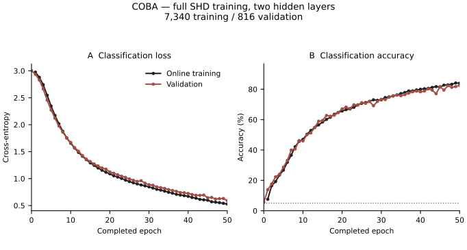
Recorded COBA training curves. We trained two 128-neuron excitatory layers on 7,340 utterances and evaluated 816 held-out utterances. (A) Example-average classification cross-entropy. (B) Classification accuracy; the dotted line marks 5% uniform random guessing across 20 classes. Black lines/circles show online pre-update minibatch measurements aggregated over each epoch; red lines/circles show complete validation with that epoch’s final weights. Epoch zero contains validation only. Each curve is one seed-42 replicate, without averaging or uncertainty bands. Class counts are naturally unequal; the split is utterance-disjoint, not speaker-disjoint.
PING training
With fixed reciprocal feedback in both 128 E/32 I layers, online training accuracy was 89% and validation accuracy 84.4% (Fig. 2B). Validation cross-entropy fell from 3.1025 to 0.4725 (Fig. 2A). All three learned matrices changed and final weights were finite. The condition took 100.8 minutes, including 91.6 minutes training and 9.2 minutes validation. It ran after COBA had completed. Higher validation accuracy in this pair does not establish a general inhibitory advantage or its mechanism.
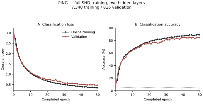
Recorded PING training curves. We used the same training/validation utterances, initial learned matrices, sample order and corruption streams as COBA. (A) Example-average classification cross-entropy. (B) Classification accuracy, with 5% uniform-guessing accuracy dotted. Black lines/circles are online pre-update measurements aggregated over the epoch; red lines/circles are full validation with final epoch weights. Epoch zero contains validation only. Each curve is one seed-42 replicate, without averaging or uncertainty bands. The official test set was not evaluated.
COBA two-layer response
We replayed the first validation utterance through the final trained weights, without optimizer updates. The true class was 0, and COBA predicted class 0. Both layers responded during the utterance (Fig. 3). This fixed example illustrates activity propagation; it was not selected for correct classification or its raster appearance and cannot summarize performance across utterances.
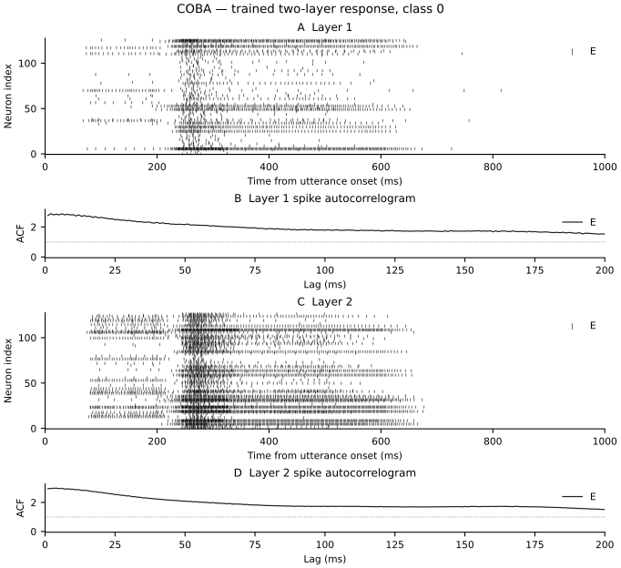
Recorded COBA inference raster. We presented one held-out SHD utterance with a fresh seeded insertion/deletion draw and fixed final-epoch weights. (A, C) Layer 1 and layer 2 rasters. Each black tick is one spike; horizontal position is elapsed time from utterance onset and vertical position identifies a neuron. Each raster contains 128 excitatory neurons and no inhibitory population. The full one-second presentation is shown, with no smoothing, trial average or transient removal. The same input events were used for PING in Figure 4. (B, D) Corresponding layer population spike-count autocorrelograms in 1 ms bins. We divided each uncentered lagged product sum by the number of overlapping bins and the squared full-utterance mean count (Equation 2). Black traces show E at positive lags up to 200 ms; zero lag is omitted because of self-pairs. The dotted line at one marks the expected baseline for independent stationary activity. These are population-count correlations, not averages of individual-neuron autocorrelations; each y axis includes the full displayed peak.
PING two-layer response
PING predicted class 0 for the same true-class-0 utterance. The raster shows intermittent excitatory responses and synchronized inhibitory events in both layers (Fig. 4). Identical inhibitory parameters and uniform incoming feedback produce identical inhibitory spike trains within a layer. This response is illustrative; the raster alone does not establish a rhythm’s frequency or show why PING trained more accurately.
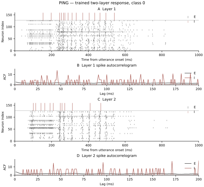
Recorded PING inference raster. We used the same utterance and corruption draw as COBA, with final-epoch weights fixed and no optimization. (A, C) Layer 1 and layer 2 rasters. Black ticks identify spikes from 128 excitatory neurons, indexed 0–127; red ticks identify spikes from 32 inhibitory neurons stacked above them, indexed 128–159. Time runs horizontally from utterance onset. The thin horizontal line separates populations. Both rasters show the full one-second presentation without smoothing, averaging or removal of the initial transient. (B, D) Corresponding population-count autocorrelograms, calculated separately for E (black) and I (red) with the same 1 ms bins, overlap correction and squared-mean normalization as Figure 3 (Equation 2). Positive lags extend to 200 ms, with zero lag omitted and no trial averaging. The dotted line at one marks the independent stationary baseline; each y axis includes both populations’ full displayed peaks. The single stimulus-evoked response includes its changing activity envelope and does not establish a sustained oscillation.
Methods
The architecture and simulation settings are listed in Table 1.
-
Prepare SHD. We split 8,156 official training utterances [1] (20 classes, 700 channels) into 7,340 training and 816 validation examples using a seed-42 per-class shuffle. Original spike-train lengths varied: last-spike times ranged from 0.233 to 1.369 s. We kept only events before 1 s to fit the simulation, flooring times into binary 1 ms bins. Speakers could overlap between splits; the official test set was unused.
-
Corrupt inputs. Per channel and 1 ms bin, we deleted existing spikes with probability 0.0008 and filled empty bins with probability 0.0016 (approximately 1.6 Hz). Both models shared example order and noise draws; validation noise stayed fixed across epochs for consistent comparison. Corruption exposed models to missing and extra spikes, but its benefit was not tested against uncorrupted training.
-
Initialize hidden weights. Both models shared seed-42 learned matrices. SNNLab’s LowerClampedNormal used parent mean 0.09 μS and SD 0.009 μS. Input→E1 and E1→E2 initial zero fractions were 0.95 and 0.90, followed by division by retained fan-in (35 and 12.8). Negative draws were clamped; initial zeros remained trainable and weights remained nonnegative.
-
Initialize readout and feedback. Signed E2→readout weights had Gaussian mean zero and SD 0.1 μS, centered across source neurons for each class, without sparsification or fan-in scaling. PING feedback was fixed at μS per E→I edge and μS per I→E edge: 0.05 μS summed incoming conductance in either direction. COBA had no inhibitory feedback.
-
Score utterances. We used a custom rate-normalized mean-voltage score:
Here is the score for class , its mean non-spiking readout voltage, and the per-neuron E2 rate, both over the full second. We used gain , reference rate and rate floor , predicting the largest score. The positive scaling preserves that choice for fixed weights but changes cross-entropy and training gradients.
-
Train both models. We used SNNLab’s train for 50 epochs with class-stratified batches of 256, merging tails smaller than 20. Custom Adam minimized mean cross-entropy per represented class; input/interlayer/readout learning rates were , with betas 0.9/0.999 and no weight decay. The FastSigmoid surrogate used slope and gradient scale 0.01. States reset per utterance. Reported losses were example means; validation used epoch-end weights, including epoch zero.
-
Record matched responses. Using SNNLab’s infer, we replayed the first validation utterance with final-epoch weights, one shared fresh corruption draw (seed 46) and no updates. Selection did not depend on prediction or spike appearance.
-
Calculate autocorrelograms. We applied SNNLab’s spike_autocorrelogram separately to each population over the full utterance:
Here is dimensionless autocorrelation for population (E or I in one layer), its count in bin , and its mean across bins. We used 1 ms bins and integer lags (1–200 ms). Independent stationary activity has baseline one; zero lag is omitted, and silent or too-short recordings give undefined curves. No smoothing, transient removal or trial averaging was applied; the stimulus-evoked activity envelope contributes to the correlation.
References
- Cramer, B., Stradmann, Y., Schemmel, J., and Zenke, F. The Heidelberg Spiking Data Sets for the Systematic Evaluation of Spiking Neural Networks. IEEE Transactions on Neural Networks and Learning Systems, 33, 2744–2757 (2022). doi:10.1109/TNNLS.2020.3044364.
Parameters
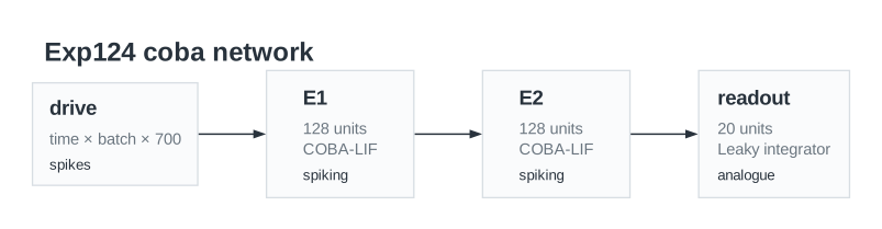
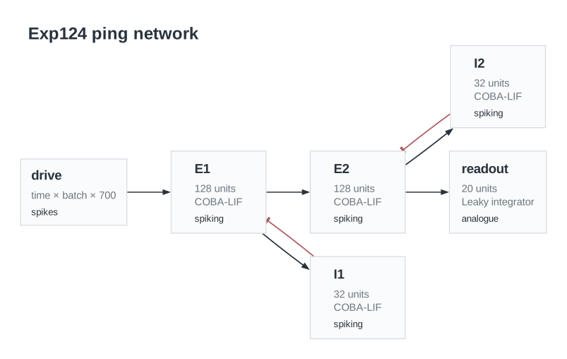
Executed network circuits. (A) COBA. (B) PING. Diagrams were generated from the retained network definitions using SNNLab’s diagram API. Boxes identify populations and their sizes; arrows show signal direction, with inhibitory connections in red. The circuit view omits measurement reductions and their output boxes; the rate-normalized readout is defined in Equation 1.
| Configuration | COBA | PING |
|---|---|---|
| Input | 700 SHD cochlear spike channels [1] | Same |
| Hidden neuron model | Conductance-based leaky integrate-and-fire (COBA LIF) | Same for both E and I |
| Synapses onto hidden neurons | Exponentially decaying AMPA conductances | Exponentially decaying AMPA and GABA conductances |
| Hidden layer 1 | 128 excitatory neurons | 128 excitatory + 32 inhibitory neurons |
| Hidden layer 2 | 128 excitatory neurons | 128 excitatory + 32 inhibitory neurons |
| Feedforward pathways | Input → E1 → E2 → readout | Same |
| Within-layer feedback | None | Fixed E→I and I→E connections in each layer |
| Readout | 20 non-spiking leaky-integrator units | Same |
| Readout synapse | Signed leaky-integrator filter, 10 ms decay | Same |
| Classification score | 20 × mean readout voltage × 20 Hz / max(mean E2 rate, 1 Hz) | Same |
| E: 1 nF | E: 1 nF; I: 0.5 nF | |
| E: 0.05 μS | E: 0.05 μS; I: 0.025 μS | |
| 20 ms (derived) | 20 ms for both E and I (derived) | |
| 10 ms | Same | |
| Not used | 10 ms | |
| Refractory period | 0 ms | 0 ms |
| Simulation timestep / presentation | 1 ms / 1 s | Same |
| Learned weights | Input→E1, E1→E2, E2→readout | Same; inhibitory feedback remains fixed |
| Training / validation utterances | 7,340 / 816 | Same |
| Epochs / batch size / seed | 50 / 256 / 42 | Same |
| Optimizer / objective | Adam / equal-class cross-entropy | Same |
| Learning rates: input / interlayer / readout | 5e-06 / 2e-05 / 0.01 | Same |
| Input insertion / deletion | 1.6 Hz per channel / 0.0008 probability | Same |
| Initial hidden weights: Gaussian parent mean / SD | 0.09 / 0.009 μS | Same |
| Initial zero fractions: input / interlayer | 0.95 / 0.9 | Same |
| Fixed summed feedback: E→I / I→E | None | 0.05 / 0.05 μS |
Architecture and simulation settings. E and I denote excitatory and inhibitory populations; E1 and E2 identify the two hidden excitatory layers. We chose a 20 ms passive time constant and fixed capacitances, then calculated leak conductances as capacitance divided by that time constant. The passive time constant is therefore derived from the configured capacitance and leak conductance, not an additional independent physical parameter. Synaptic conductances change the effective membrane time constant. AMPA and GABA time constants describe conductance decay. Readout voltage and E2 firing rate are averaged over each one-second utterance. Neuronal and synaptic states reset between utterances.
Dataset
Upstream: —
Downstream: —
| Run | Date | Duration | Size | Ran on | Source |
|---|---|---|---|---|---|
| exp124-r164-presentUsed | 1s | 550.1 KB | Local | Local (6) | |
| exp124-r162-analyseUsed | 1s | 95.5 KB | Local | Local | |
| exp124-r149-computeUsed | <1s | 176.8 MB | Local | Local |