Introduction to Spiking Neural Networks
A practical introduction to neurons, temporal computation, and learning for machine learning practitioners and software developers.
Abstract
An introduction to spiking neural networks for machine learning practitioners and software developers. Interactive demonstrations explore how a neuron accumulates input and fires, how synaptic weights combine inputs, and how supervised learning changes a small classifier. In one run, validation-selected held-out accuracy rose from 50% to 100% on 128 examples. A training replay highlights a short stretch of the full loss curve. The examples use a synthetic two-class task.
Introduction
A leaky integrate-and-fire neuron’s input current charges its membrane capacitance . The membrane voltage leaks towards rest , with time constant ; is time.[1]
Each input pulse starts at , supplies current , and lasts one simulation timestep . Overlapping pulses add; between pulses the input current is zero.
Reaching the firing threshold produces a spike.
The voltage then returns immediately to the reset value .
Here, pF and ms. Rest and reset are −65 mV, and threshold is −50 mV. Currents are in nA, voltages in mV, and times in ms. There is no refractory period.
Loading neuron…
Synapses
A synapse connects a presynaptic neuron to a postsynaptic neuron. Its weight sets how strongly an arriving spike affects the receiving neuron.[2] In this simplified current-based model, the inputs add:
is the number of presynaptic neurons; is the current-pulse amplitude per spike from neuron , in nA. The spike count counts its arrivals during simulation step , usually 0 or 1. Multiple arrivals contribute separately. The sum is the total current applied throughout that step.
Three independent Poisson spike trains encode rates of 40, 30, and 20 Hz below. These are mean spikes per second, with random exponentially distributed waiting times.[3] Change a weight to change that connection’s contribution; zero removes it. Each arriving spike supplies a rectangular current pulse, without detailed biological synaptic dynamics.
Loading neuron…
Results
Training
The classifier learns which of its first two inputs has the higher Poisson firing rate; a third supplies background spikes. We trained six nonnegative weights between three input channels and two spiking output neurons. Cross-entropy used their output spike counts. The forward pass retained the hard firing threshold; backpropagation used a smooth surrogate derivative to propagate learning signals through it.[4]
Training follows a loop: run the inputs forward, compare the output spike counts with the correct classes, calculate gradients, and update the weights. A gradient describes how a small weight change would affect the loss; it is a calculation, not a spike travelling backwards.
The animation uses a separate teaching run: 48 updates on the same batch of 128 training examples. The full graph shows the batch loss, while the network shows one example from that batch. Eight consecutive updates from the stretch with the largest loss decrease are replayed slowly. Weight changes and gradients are recorded; their motion is illustrative.
Loading training…
Inference
Once trained, the classifier runs inputs forward with fixed weights to make a prediction. The output with more spikes wins; ties are assigned to Class A.
Training used 128 examples, with 64 separate validation examples selecting the checkpoint. On 128 held-out examples, accuracy increased from 50% to 100%. Toggle Before Training / After Training to compare the same recorded input. Before training, both outputs respond equally and fail to discriminate; training changes their relative responses. This is one training run on a synthetic task.
Loading classifier…
Network diagrams
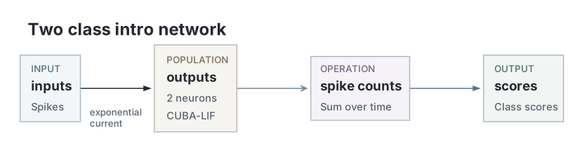
Circuit view rendered from the original compute’s saved classifier bundle. The teaching loop and validation-selected classifier share this architecture; their learned weights differ. The presentation reuses the original recordings.
Parameters
| Parameter | Recorded value |
|---|---|
| Network | |
| Native parameter snapshot | Unavailable |
| Input channels | Unavailable |
| Populations | Unavailable |
| Membrane model | Unavailable |
| Neurons | |
| Membrane capacitance | Unavailable |
| Leak conductance | Unavailable |
| Resting potential | Unavailable |
| Reset potential | Unavailable |
| Threshold | Unavailable |
| Refractory period | Unavailable |
| Membrane time constant | Unavailable |
| Synapses and weights | |
| Native synapse and weight parameters | Unavailable |
| Input and simulation | |
| Seed | 127 |
| Timestep | 1 ms |
| Presentation duration | 200 ms |
| Training / validation / test samples | 128 |
| Validation samples | 64 |
| Held-out test samples | 128 |
| Input encoding | independent Poisson counts in 1 ms bins, clipped to binary occupancy for SNNLab spike inputs |
| Rate patterns | [[125,12.5,31.25],[12.5,125,31.25]] Hz |
| Rate jitter multipliers | [0.85,1.15] |
| Checkpoint selection | minimum validation cross-entropy, earliest epoch on ties, including initial |
| Readout | total output spike counts over 200 ms; ties choose class A |
| Replay selection | first held-out example of each class, independent of model responses |
| Training | |
| Epochs | 24 |
| Batch size | 64 |
| Learning rate | 0.02 |
| Surrogate slope | 1 |
| Gradient clipping | 5 |
| Teaching updates | 48 |
| Teaching replay window | 8 |
| Analysis | |
| Selected epoch | 24 |
| Decision minimum spikes / lead | 5 / 3 |
| Teaching replay selection | Consecutive window with the greatest recorded batch-loss decrease |
Dataset
Upstream: —
Downstream: —
| Run | Date | Duration | Size | Evidence | Storage | Ran on | Verification |
|---|---|---|---|---|---|---|---|
| exp127-r015-present | <1s | 460.6 KB | Current | R2 | Local | Local: absent; R2: catalog-verified | |
| exp127-r013-analyse | <1s | 44.5 KB | Current | R2 | Local | Local: absent; R2: catalog-verified | |
| exp127-r012-compute | 3s | 741.5 KB | Current | R2 | Local | Local: absent; R2: catalog-verified |
References
- W. Gerstner, W. M. Kistler, R. Naud, and L. Paninski. Neuronal Dynamics: From Single Neurons to Networks and Models of Cognition. Cambridge University Press (2014), §1.3, “Integrate-And-Fire Models.”
- W. Gerstner, W. M. Kistler, R. Naud, and L. Paninski. Neuronal Dynamics: From Single Neurons to Networks and Models of Cognition. Cambridge University Press (2014), §3.1, “Synapses.”
- W. Gerstner, W. M. Kistler, R. Naud, and L. Paninski. Neuronal Dynamics: From Single Neurons to Networks and Models of Cognition. Cambridge University Press (2014), §7.5, “Renewal statistics.”
- E. O. Neftci, H. Mostafa, and F. Zenke. “Surrogate Gradient Learning in Spiking Neural Networks.” arXiv (2019). arXiv:1901.09948