Output Evidence Against Time and Gamma Cycles
Paired inhibitory-decay probes of output evidence, matched-coordinate accuracy and accuracy–deadline–spike-cost frontiers across input encoding rates.
Abstract
We examine how output evidence accumulates in a trained pyramidal–interneuron gamma (PING) network when inhibitory decay changes. With network weights fixed, paired MNIST spike encodings are presented at inhibitory decay times of 3, 6 and 12 ms. We compare cumulative output-spike scores against elapsed time and completed inhibitory volleys, then assess sustained correct decisions and classification accuracy at matched time, cycle and input-spike coordinates. Across three encoding rates, we also compare accuracy, decision deadlines and network spike cost, identifying empirical Pareto candidates. These comparisons examine whether volley count provides a useful coordinate for evidence accumulation. Softmax scores are uncalibrated, later coordinates select trial subsets, and spike cost is not a measure of physical energy.
Background
We imported the trained PING network from exp022 — Training Runs and kept its weights fixed. The parameter table lists the network and simulation settings.
Evidence across time
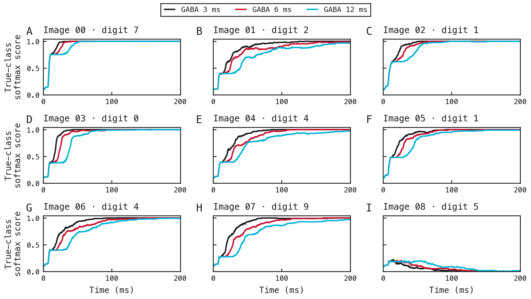
A–I each show one of the first nine MNIST test images. We converted each image into 100 random spike trains, with brighter pixels having higher average spike rates (25 spikes per second for a fully bright pixel). Each train was presented for 200 ms to the same trained network with fixed weights, using three inhibitory decay times: 3 ms (black), 6 ms (red) and 12 ms (cyan). The x-axis shows elapsed time. The y-axis shows the score assigned to the correct digit, calculated by applying softmax to accumulated output spike counts. Each curve averages the 100 trials; no uncertainty bands are shown. This score is not a calibrated probability of being correct.
We encoded each of the first nine MNIST test images into 100 random spike trains and reused each train at ms, where is the inhibitory decay time constant. Brighter pixels had higher average spike rates, with 25 spikes per second for a fully bright pixel. Each presentation lasted 200 ms, with 0.1 ms simulation steps. For each trial, the logit for digit was its accumulated output spike count:
Here, is elapsed time, is the timestep, indexes simulation steps, and is one when output neuron spikes, otherwise zero. We converted these logits into scores using softmax:
Here, is the score for digit , and ranges over all ten digits. We averaged the correct digit’s score after softmax across 100 trials, separately for each decay setting. These scores are uncalibrated.
Evidence per completed volley
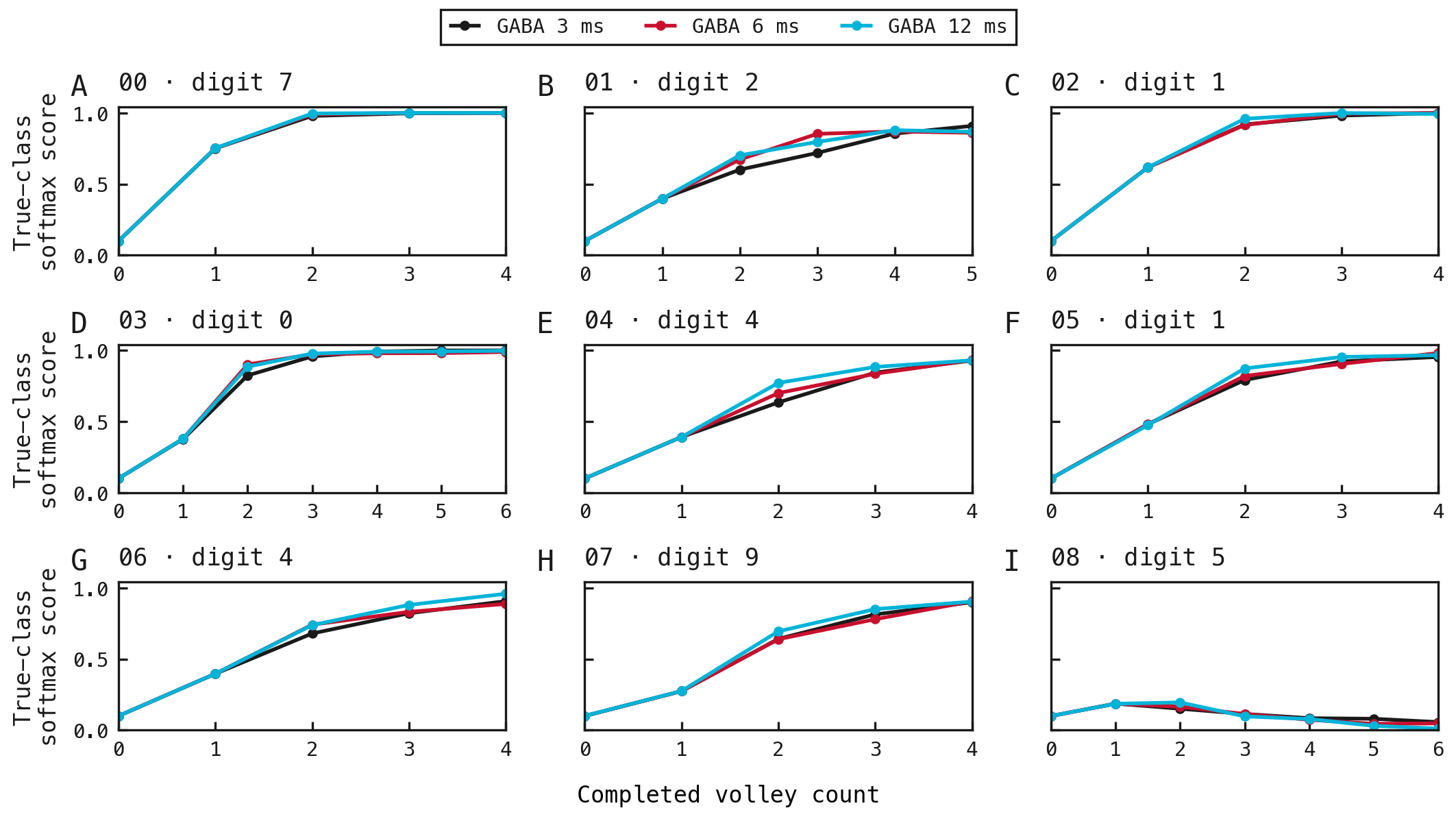
A–I: the same nine MNIST test images, using the score definition and colours of Figure 1. Each point samples the cumulative score at the inhibitory trough after the numbered volley, then averages across 100 trials. The trough is the minimum of smoothed I activity between successive accepted peaks; the final peak is excluded because it has no following boundary. Volley zero shows the initial score of 0.1 at time zero, not a detected volley. Only counts available in every trial and setting are shown; lines connect integer counts without representing elapsed time. Clustering and score saturation can mimic alignment.
We detected inhibitory peaks after 1 ms Gaussian smoothing, requiring ≥2 ms spacing and prominence ≥max(1 spike, 20% of the maximum). Accepted sequences required a complete interior cycle and mean inhibitory participation ≥50%.
We defined each volley’s completion as the minimum of smoothed inhibitory activity between its peak and the next. At that boundary, we sampled the correct digit’s softmax score from all output spikes accumulated since onset.
We averaged these samples across 100 trials for each decay setting, using completed-volley counts available in every trial and setting. The final unbounded volley is excluded; count zero shows the initial score of 0.1 at time zero, not a detected volley. Clustering and score saturation can mimic alignment.
Sustained correct decisions
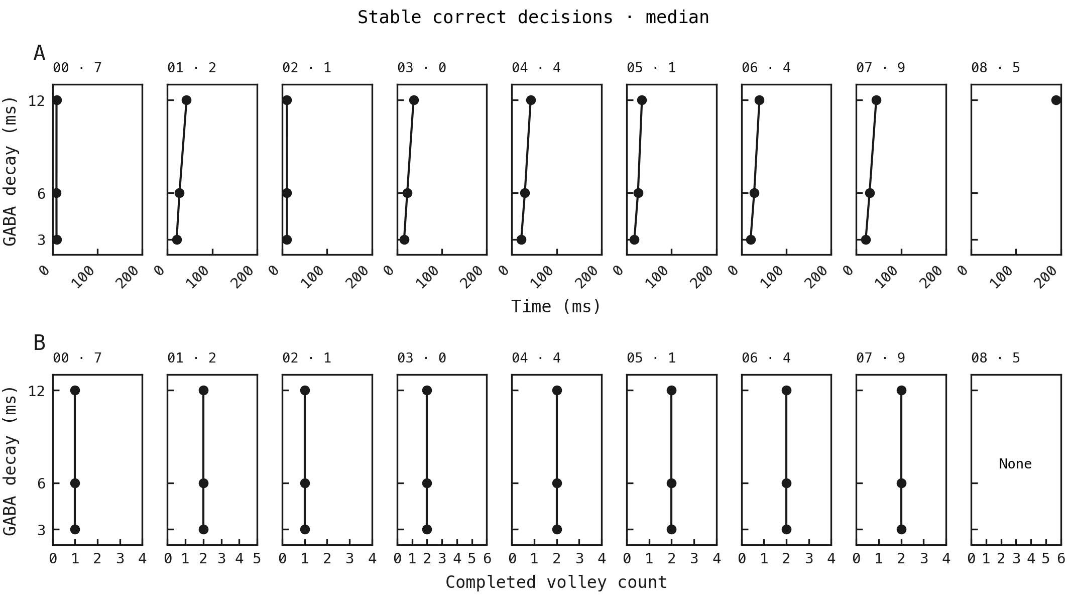
A: time (ms). B: completed volley count, using the inhibitory trough boundaries of Figure 2. B uses the first completion at which the decision is already stable. Both rows show GABA decay on y for images 00–08. Each point is the median among trials whose correct digit becomes the unique winner and stays so through 200 ms. Lines connect the three decay settings. Failed trials are excluded; B also requires completion-boundary coverage within Figure 2’s shared count range. Trial counts are integers; medians can be fractional.
For the same nine images and 100 trials per decay setting, we found the earliest update at which the correct digit had the largest cumulative output spike count and remained the unique winner through 200 ms. Ties interrupt stability; trials without a stable correct decision were excluded.
We used the first completed-volley trough boundary at or after each stable decision. This is the first sampled point at which the decision is already stable, numbered from one. Counts required accepted volley sequences, a decision no later than the final completion boundary, and the shared completed-volley count range. We summarised median decision time and median completed-volley count against inhibitory decay. The two summaries can include different trial subsets. Trial counts are integers; medians can be fractional. Stability was assessed retrospectively, not by a stopping rule.
Accuracy at matched coordinates
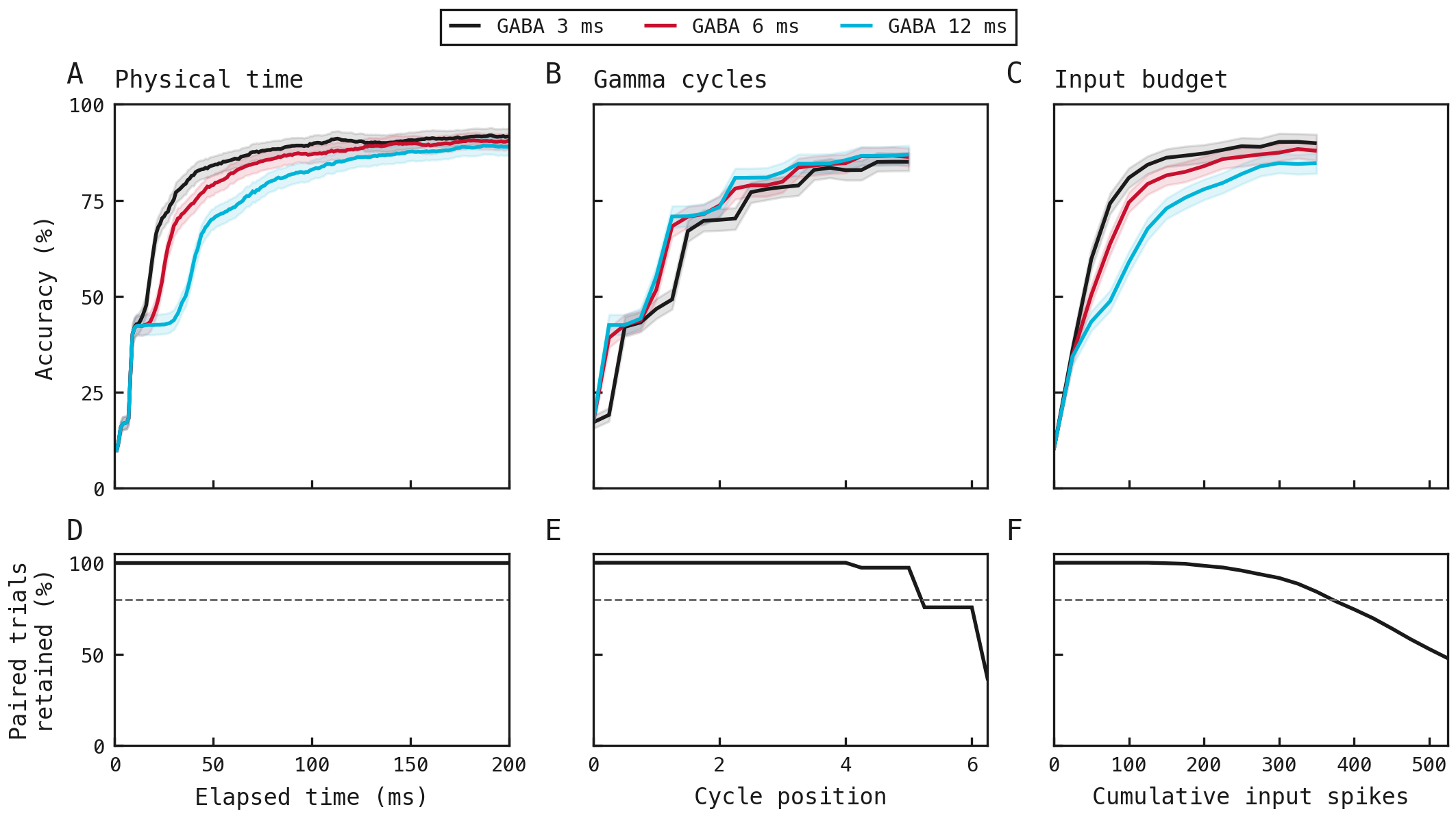
A–C: accuracy against time, cycle position and cumulative input spikes. D–F: paired-trial coverage. Sample: 500 images, 50 per digit, three paired encodings; decay 3/6/12 ms in black/red/cyan. Shading: image-bootstrap 95% intervals. Dashed lines mark 80% coverage; accuracy is omitted below it. Later coordinates select subsets. Equal spike counts do not guarantee equal information.
We compared accuracy against time, cycle position and cumulative input spikes, alongside paired-trial coverage. The sample comprised 500 images, 50 per digit, with three paired encodings and inhibitory decay times of 3, 6 and 12 ms. Uncertainty was summarised with image-bootstrap 95% intervals. Accuracy is omitted below 80% coverage. Later coordinates select subsets. Equal spike counts do not guarantee equal information.
Accuracy and spike cost
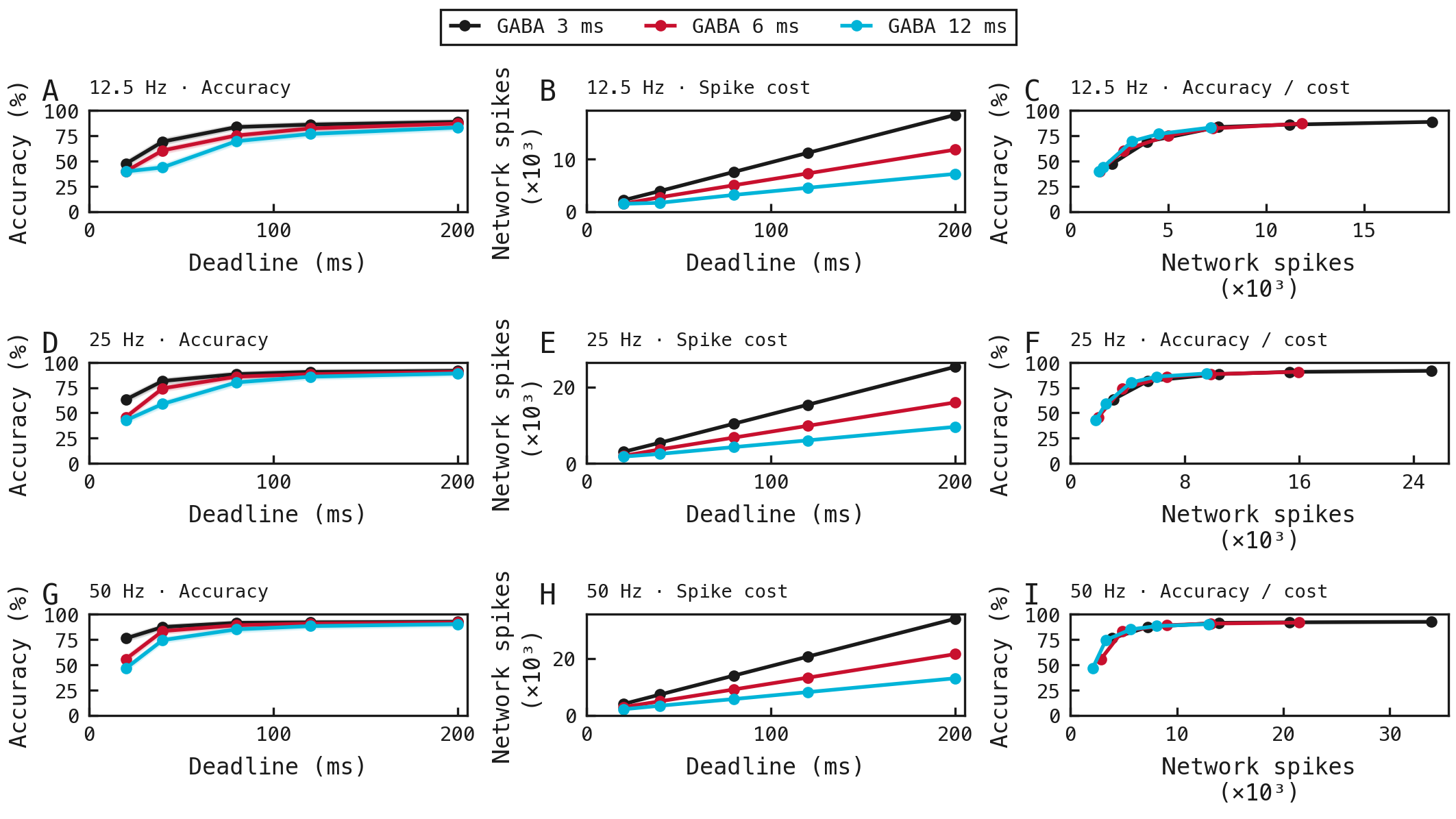
A/D/G: accuracy versus deadline. B/E/H: mean network spikes versus deadline. C/F/I: accuracy versus spike cost. Rows: 12.5/25/50 Hz encoding; colours: 3/6/12 ms decay. Points mark five deadlines, connected within each setting. Sample: 500 images, three paired encodings. Shading in A/D/G: image-bootstrap 95% intervals. Cost includes E, I and output spikes, excluding input. Spike cost is not physical energy; encoding rate also changes drive.
We compared accuracy versus deadline, mean network spikes versus deadline, and accuracy versus spike cost at encoding rates of 12.5, 25 and 50 Hz and inhibitory decay times of 3, 6 and 12 ms. We evaluated five deadlines within each setting, using 500 images and three paired encodings. Accuracy uncertainty was summarised with image-bootstrap 95% intervals. Cost includes excitatory, inhibitory and output spikes, excluding input. Spike cost is not physical energy; encoding rate also changes drive.
Pareto candidates and frequency
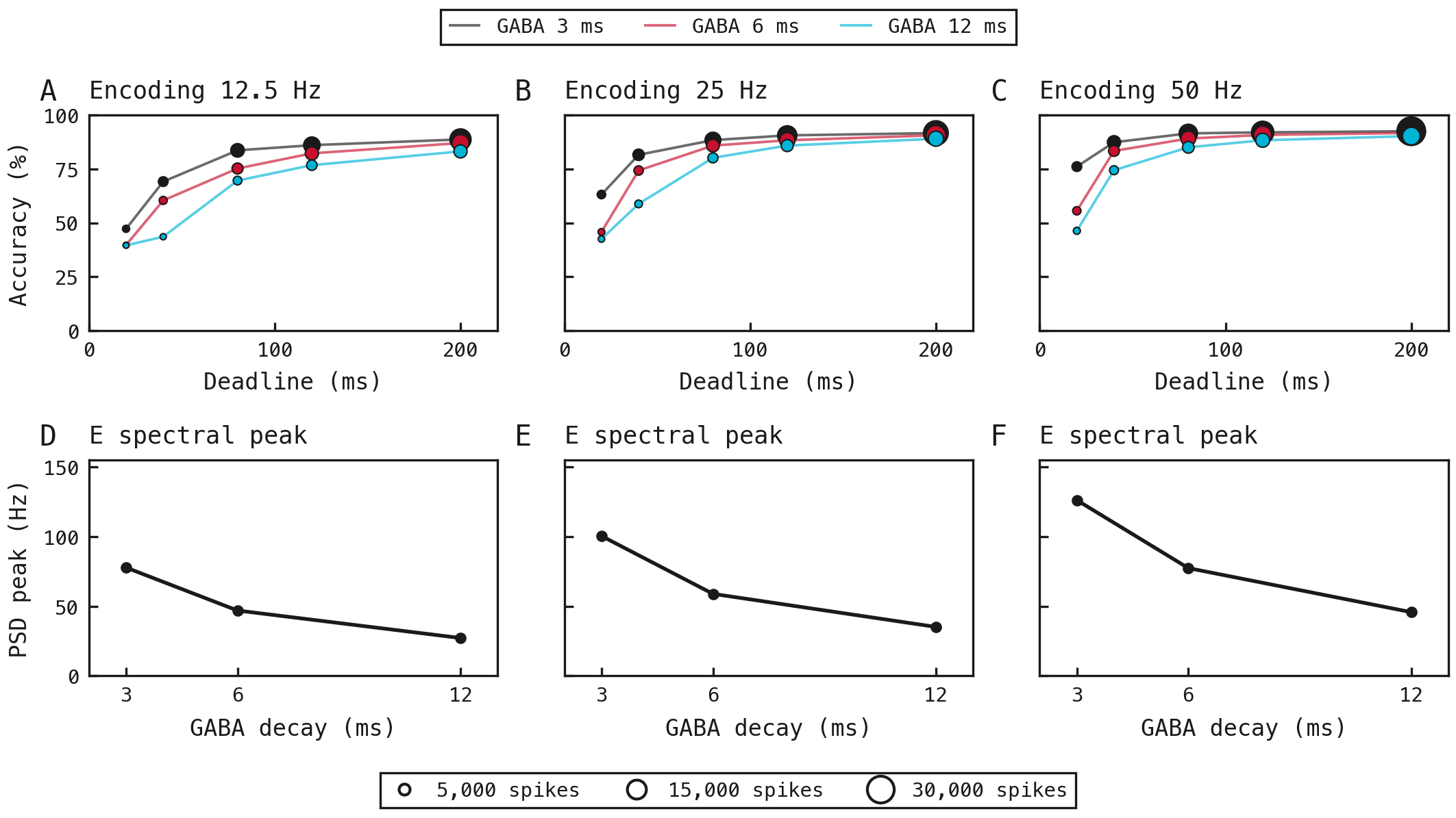
A–C: Pareto comparisons at 12.5/25/50 Hz encoding. Position shows deadline and accuracy; bubble area shows mean network spikes on a common scale. Colours identify decay; traces connect deadlines. Outlined bubbles are empirically nondominated; faint bubbles are dominated. D–F: peaks of mean E-population PSDs at the same rates. Peaks can reflect harmonics or heterogeneous rhythms. Sample and cost definition: Figure 5. Frontier membership is sample-dependent.
We compared Pareto candidates using deadline, accuracy and mean network spikes at encoding rates of 12.5, 25 and 50 Hz, for each inhibitory decay setting. Candidates were classified as empirically nondominated or dominated. Frontier membership is sample-dependent.
We also measured peaks of mean excitatory-population power spectral densities at the same encoding rates. Peaks can reflect harmonics or heterogeneous rhythms. The sample and cost definition were the same as in the accuracy and spike-cost comparison.
Parameters
| Parameter | Value |
|---|---|
| Population sizes | Input: 784; E: 1,024; I: 256; output: 10 |
| Capacitance | E: 1.0 nF; I: 0.5 nF |
| Leak conductance | E: 0.05 µS; I: 0.10 µS |
| Rest and reset voltage | E and I: −65 mV |
| Spike threshold | E and I: −50 mV |
| Refractory hold | E: 1.2 ms; I: 0.6 ms |
| AMPA decay | 2 ms |
| Inhibitory decay sweep | 3, 6 and 12 ms |
| Reciprocal projection delay | One simulation step (0.1 ms) |
| Input filter and output leak | 2 ms each |
| Output threshold and reset | Threshold 1; subtractive reset |
| Simulation step and duration | 0.1 ms; 200 ms; no burn-in |
| Input encoding rates | 12.5, 25 and 50 Hz |
| Frozen weights | Final epoch after 50 training epochs; training seed 42; directly reused without selection or fitting here |
| Initial state per presentation | Hidden neurons at rest; conductances and output state zero |
| Encoding generator seed | 1,000 × image index + draw identifier |
Dataset
Figures use the latest presentation run and their same-experiment inputs. The table includes completed run history; the presentation used by this report is emphasized. Dates are run creation times in UTC; durations cover each stage separately, and sizes cover its exported files. For imported runs, durations and execution locations refer to the recorded producing execution.
Upstream: exp022 — Training Runs
Downstream: —
| Run | Date | Duration | Size | Ran on |
|---|---|---|---|---|
| exp123-r052-present | 2s | 4.5 MB | Local | |
| exp123-r051-present | 2s | 4.5 MB | Local | |
| exp123-r050-present | 2s | 4.5 MB | Local | |
| exp123-r049-analyse | 1m | 38.9 MB | Local | |
| exp123-r048-analyse | 1m 6s | 38.9 MB | Local | |
| exp123-r047-present | 5s | 4.4 MB | Local | |
| exp123-r046-analyse | 1m 23s | 38.8 MB | Local | |
| exp123-r045-present | 3s | 4.4 MB | Local | |
| exp123-r044-present | 2s | 4.4 MB | Local | |
| exp123-r043-analyse | 59s | 38 MB | Local | |
| exp123-r042-present | 2s | 4.4 MB | Local | |
| exp123-r041-analyse | 1m 2s | 38 MB | Local | |
| exp123-r040-compute | 8m 14s | 211.9 MB | Local |